


Abstract
Sophisticated inferential tools coupled with the coalescent model have recently emerged for estimating past population sizes from genomic data. Recent methods that model recombination require small sample sizes, make constraining assumptions about population size changes, and do not report measures of uncertainty for estimates. Here, we develop a Gaussian process-based Bayesian nonparametric method coupled with a sequentially Markov coalescent model that allows accurate inference of population sizes over time from a set of genealogies. In contrast to current methods, our approach considers a broad class of recombination events, including those that do not change local genealogies. We show that our method outperforms recent likelihood-based methods that rely on discretization of the parameter space. We illustrate the application of our method to multiple demographic histories, including population bottlenecks and exponential growth. In simulation, our Bayesian approach produces point estimates four times more accurate than maximum-likelihood estimation (based on the sum of absolute differences between the truth and the estimated values). Further, our method’s credible intervals for population size as a function of time cover 90% of true values across multiple demographic scenarios, enabling formal hypothesis testing about population size differences over time. Using genealogies estimated with ARGweaver, we apply our method to European and Yoruban samples from the 1000 Genomes Project and confirm key known aspects of population size history over the past 150,000 years.
FOR a single nonrecombining locus, neutral coalescent theory predicts the set of timed ancestral relationships among sampled individuals, known as a gene genealogy (Kingman 1982; Hudson 1983, 1990; Tajima 1983). In the coalescent model with variable population size, the rate at which two lineages have a common ancestor (or coalesce) is a function of the population size in the past. Here we denote the population size trajectory by where t is time in the past, and use the term local genealogy to describe ancestral relationships at one nonrecombining locus. When analyzing multilocus sequences, a single local genealogy will not represent the full history of the sample. Instead, the set of ancestral relationships and recombination events among a sample of multilocus sequences can be represented by a graph, known as the ancestral recombination graph (ARG), which depicts the complex structure of neighboring local genealogies and results in a computationally expensive model for inferring (Griffiths and Marjoram 1997; Wiuf and Hein 1999).
Recent studies have leveraged approximations for the coalescent with recombination—the sequentially Markov coalescent (SMC) (McVean and Cardin 2005) and its variant SMC′ (Marjoram and Wall 2006; Chen et al. 2009)—both of which model local genealogies as a continuous-time Markov process along sequences (Figure 1). The difference between the SMC and the SMC′ is that the SMC models only the class of recombination events that alter local genealogies of the sample; in general, the SMC′ is a better approximation to the ARG than the SMC (Chen et al. 2009; Wilton et al. 2015). Because of these features, in this work we rely on the SMC′ to model local genealogies with recombination.
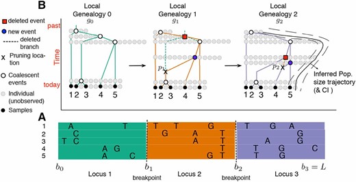
SMC′ hidden Markov model for inferring population size trajectories, drawn according to Rasmussen et al. (2014) to highlight notation specific to our study. (A) Observed sequence data in a segment of length L from five individuals. Three loci are shown delimited by recombination breakpoints and . Only the derived mutations at polymorphic sites are shown. (B) Corresponding local genealogies for each locus i. The five sampled individuals are depicted as solid black circles. Local genealogies have a Markovian degree-1 dependency. Each intercoalescent time (the time interval between coalescent events denoted as open circles) provides information about past population size (number of solid gray circles at a given time point). Moving from left to right after recombination breakpoint the pruning location is selected from genealogy and the pruned branch is regrafted back on the genealogy (solid blue circle). The coalescent event of depicted as a solid red circle in is deleted. This creates the next genealogy . The process continues until L. At L, the population size trajectory (depicted as a black curve superimposed on ) can be inferred.
Under the coalescent and SMC′ models, population size trajectories and sequence data are separated by two stochastic processes: (i) a state process that describes the relationship between the population size trajectory and the set of local genealogies and (ii) an observation process that describes how the hidden local genealogies are observed through patterns of nucleotide diversity in the sequence data. The observation process includes mutation and genotyping error while the state process models coalescence. Population size trajectories are then inferred from sequence data, using these coalescent-based hidden Markov models. In this study, we restrict attention to the state process and present a novel Bayesian approach for inferring population size trajectories from local genealogies. We solve a number of key modeling and inference problems and thus provide a basis for developing efficient algorithms to infer population parameters from sequence data directly.
Whole-genome inference of population size trajectories has been hampered by the enormous state space of local genealogies for large sample sizes. The pioneering pairwise sequentially Markov coalescent (PSMC) method of Li and Durbin (2011) employed the SMC to infer from a sample of size 2 (). In this method, time is discretized and the population size trajectory is piecewise constant. Subsequent methods for samples larger than 2 similarly rely on the discretization of time. The natural extension of the PSMC to is the multiple sequentially Markovian coalescent (MSMC) (Schiffels and Durbin 2014). However, the MSMC models only the most recent coalescent event of the sample; thus MSMC’s estimation of population sizes is limited to very recent times. Other recent methods propose efficient ways of exploring the state space of hidden genealogies for (Sheehan et al. 2013; Rasmussen et al. 2014), yet also rely on discretizing the state space of local genealogies and assume a piecewise constant trajectory of population sizes.
Gaussian process-based Bayesian inference of population size trajectories has proved to be a powerful and flexible nonparametric approach when applied to a single local genealogy (Palacios and Minin 2013; Lan et al. 2015). The two main advantages of the Gaussian process (GP)-based approach are (i) it does not require a specific functional form of the population size trajectory (such as constant or exponential growth) and (ii) it does not require an arbitrary specification of change points in a piecewise constant or linear framework.
In this article, we overcome the limitations of existing methods—discretizing time, assuming a piecewise constant trajectory, and reporting only point estimates for past population sizes—by introducing a Bayesian nonparametric approach with a GP to model the population size trajectory as a continuous function of time. More specifically, we model the logarithm of the population size trajectory a priori as a Gaussian process (the log ensures our estimates are positive). As mentioned above, we assume that local gene genealogies are known. For our Bayesian approach, we develop a Markov chain Monte Carlo (MCMC) method to sample from the posterior distribution of population sizes over time. Our MCMC algorithm uses the recently developed algorithm, split Hamiltonian Monte Carlo (splitHMC) (Shahbaba et al. 2014; Lan et al. 2015). To compare our Bayesian GP-based estimation of population size trajectories with a piecewise constant maximum-likelihood-based estimation (e.g., Li and Durbin 2011; Sheehan et al. 2013; Schiffels and Durbin 2014), we implement the expectation-maximization (EM) algorithm within our framework and compute the observed Fisher information to obtain confidence intervals of the maximum-likelihood estimates.
Finally, we address a key problem for inference of population size trajectories under sequentially Markov coalescent models: the efficient computation of transition densities needed in the calculation of likelihoods. Here, we express the transition densities of local genealogies in terms of local ranked tree shapes (Tajima 1983) and coalescent times and show that these quantities are statistically sufficient for inferring population size trajectories either from sequence data directly or from the set of local genealogies. The use of ranked tree shapes allows us to exploit the state process of local genealogies efficiently since the space of ranked tree shapes has a smaller cardinality than the space of labeled topologies (Sainudiin et al. 2014).
Methods: SMC′ Calculations
Following notation similar to that in Rasmussen et al. (2014) (Table 1), a realization of the embedded SMC′ chain consists of a set of m local genealogies recombination breakpoints at chromosomal locations and pruning locations where indicates the time of the recombination event and the branch where recombination happened in genealogy (Figure 1). Genealogy corresponds to the genealogy of n sequences that contains the set of timed ancestral relationships among the n individuals for the chromosomal segment . Genealogy corresponds to the genealogy of the same n sequences for the chromosomal segment for . Finally, denotes the time when two of j lineages coalesce in genealogy measured in units of generations before present.
Notation for the SMC′ model used in this work
| Symbol | Description |
|---|---|
| Parameters | |
| ρ | Recombination rate per site per generation |
| Effective population size trajectory with time measured in units of generations | |
| τ | Hyperparameter that controls the smoothness of the log-Gaussian process prior on |
| Notation specific to SMC′ chain | |
| L | Length of observed sequences |
| Chromosomal location of the ith recombination breakpoint | |
| m | No. local genealogies corresponding to recombination events |
| Segment length for local genealogy i | |
| Local genealogy for the segment | |
| Notation specific to local genealogy | |
| n | Sample size or no. sequences |
| Total tree length of local genealogy | |
| Piecewise constant function of the number of ancestral lineages at time t in local genealogy | |
| Coalescent time in genealogy when two of j lineages coalesce. | |
| Vector of coalescent times of genealogy | |
| Pruning location along local genealogy | |
| Time when the recombination event happened along the height of the genealogy | |
| Lineage on genealogy where the recombination event happened | |
| New lineage added on genealogy where the recombination event happened | |
| Coalescent time in genealogy when the lineage coalesces | |
| Coalescent time in genealogy that no longer exists in genealogy | |
| Lineage on genealogy that coalesces with lineage | |
| No. free lineages in local genealogy that do not coalesce in the time interval | |
| Piecewise constant function that takes values in indicating no. ancestral lineages at time t in genealogy where the pruning event would produce a visible transition to | |
| Discretization | |
| d | No. change points at which is estimated |
| Times at which is estimated |
Complete data transition densities
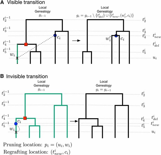
Schematic representation of SMC′ transitions given a recombination breakpoint at location (indicated as an arrow in each panel). (A) Visible transition. We uniformly sample the pruning location from at time along some branch and we add a new branch at and regraft it (dashed black line). The new branch coalesces with some branch at time . We then delete branch and the coalescent time to generate genealogy . Any pruning time along the branch (shown in green) would have produced the same visible transition from to . (B) Invisible transition. We uniformly sample the pruning location add a new branch at and regraft it. The new branch coalesces with itself (dashed black line), that is, and then the segment of is deleted. If any pruning location along the green branches would have produced the same invisible transition.
This generative process for local genealogies can result in a visible transition, where a genealogy is different from (Figure 2A), or an invisible transition, where is identical to (Figure 2B).
Transition densities averaged over unknown pruning locations
Even though we assume that local genealogies are known, to build inferential frameworks for sequence data in the future, we do not wish to make the same assumption about pruning locations. Thus, we average over pruning locations to obtain marginal transition densities between genealogies for both visible and invisible transitions.
Visible transitions:
To compute the marginal visible transition density to a new genealogy we need to average over all possible pruning locations along . By comparing the two genealogies and in Figure 2A, we know that corresponds to the lineage some time along or, equivalently, along . In general, comparison of and may not provide complete information to identify the lineage that was pruned. When the children of the node corresponding to and the children of the node corresponding to are the same, pruning different branches can lead to the same transition. We enumerate all cases of incomplete information for visible transitions in Supporting Information, File S1, and File S2.
Invisible transitions:
To compute the marginal transition probabilities for invisible events, we must average over all possible pruning locations . Consider the example in Figure 2B and choosing a pruning time () along . To have an invisible transition, the coalescing branch must be the same pruning branch . In Figure 2B the new coalescent time can happen along five lineages in the interval three lineages in the interval and two lineages in the interval . To generalize this calculation, we introduce the quantity with which denotes the number of lineages in that are free (do not coalesce), in the time segment with The time interval includes the interval of pruning up to the interval of self-coalescence . Thus, if the pruning time happens at time an invisible transition with new coalescent time can happen along free lineages.
The likelihood of the embedded SMC′ chain
Methods: Inference
In the following sections, we first present our Bayesian nonparametric method and then develop a maximum-likelihood method under a piecewise constant trajectory so we can directly compare an EM-based method to our Bayesian nonparametric method.
Gaussian-process-based Bayesian nonparametric estimation of
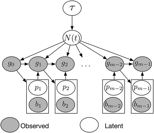
Structure of our Bayesian model for inferring population size trajectories from a realization of the SMC′ process at recombination breakpoints. Hyperparameter τ controls the smoothness of the log-Gaussian process prior on . Local genealogies depend on and form a Markov chain of degree 1. Given the current local genealogy we sample the location of the new recombination breakpoint and a pruning location on genealogy . The new genealogy depends on and .
Alternatively, one can update in the MCMC algorithm, using the elliptical slice sampler (Murray et al. 2010) with a fixed value of τ (perhaps estimated from previous studies or from a preliminary run from the split Hamiltonian Monte Carlo algorithm). The advantage of using the elliptical slice sampler over the split Hamiltonian Monte Carlo is purely computational (the elliptical slice sampler does not require calculation of the score function).
Maximum-likelihood estimation of with measures of uncertainty
We assume that the population size trajectory is defined as in Equation 14. The standard coalescent density (Equation 4) and the transition densities defined in Equations 8 and 11 are tractable, so calculation of the likelihood (Equation 13) is tractable. However, maximization of the likelihood function cannot be performed analytically because pruning locations are missing. We implement an EM algorithm (Dempster et al. 1977) to find the maximum-likelihood estimator of . The complete data for inferring are then the set of local genealogies and the set of pruning locations . For the invisible transitions, we also need to know the new coalescent times where denotes the set of indexes of invisible transitions.
Data availability
The R code for all simulation studies and analysis of sequence data conducted in this article are publicly available at http://ramachandran-data.brown.edu/.
Results
We simulated 1000 local genealogies of 2, 20, and 100 individuals from each of the three different demographic models described in Table 2, using MaCS (Chen et al. 2009); see File S3 for details of these simulations. We assumed that all individuals were sampled at time
Simulated demographic scenarios
| Demographic model | |
|---|---|
| Constant population size | |
| Exponential growth followed by constant size | |
| Population bottleneck |
| Demographic model | |
|---|---|
| Constant population size | |
| Exponential growth followed by constant size | |
| Population bottleneck |
The argument t denotes time measured in units of generations.
| Demographic model | |
|---|---|
| Constant population size | |
| Exponential growth followed by constant size | |
| Population bottleneck |
| Demographic model | |
|---|---|
| Constant population size | |
| Exponential growth followed by constant size | |
| Population bottleneck |
The argument t denotes time measured in units of generations.
For our Bayesian GP estimates, we estimate at time points, unless stated otherwise.
The parameters of the Gamma prior on the GP precision parameter τ were set to reflecting our lack of prior information about the smoothness of the population size trajectory.
For our EM estimates, we used different discretizations based on Equation 15 and varying the number of change points d and κ over the fixed interval with set to be the maximum observed coalescent time. For the cases where we consider only one genealogy (), the EM approach becomes standard maximum-likelihood estimation.
We summarize our posterior inference and compare our Bayesian GP method to the EM method in Figure 5, Figure 6, and Figure 7. The population size trajectory is log-transformed for ease of visualization and for direct comparison with other methods (Minin et al. 2008; Palacios and Minin 2013).
Sensitivity of EM estimates of to discretization
In Figure 4, we show our Bayesian GP and EM estimates of a constant population size trajectory from a single genealogy of 100 individuals with different discretizations. We find that our Bayesian GP point estimates depicted in Figure 4A recover the truth (dashed line) almost perfectly with less uncertainty than the EM (Figure 4, B and C). Comparing our Bayesian GP estimates with different discretizations [50, 100, and 200 equally spaced time points (Figure 4A)], we find that increasing the number of time points improves inference (Table 3) but that the differences between estimates among the three discretizations are marginal (Figure 4A). In contrast, we show that different grid definitions alter the EM estimates (Figure 4B). It is not clear how to define a good strategy for the definition of the grid for the EM method, even for the simple model of constant population size. For example, increasing κ from 100 to 500 with 5 change points (Figure 4B) does not improve estimation. Increasing the number of change points does not necessarily improve the estimates either, for example, increasing the number of change points from 5 to 10 for (Figure 4, B and C). EM grid sensitivity is persistent even when the number of genealogies increases; Figure S2 in File S4 shows that the best definition of change points when our data consist of 1000 local genealogies of 100 individuals is 10 evenly distributed change points.
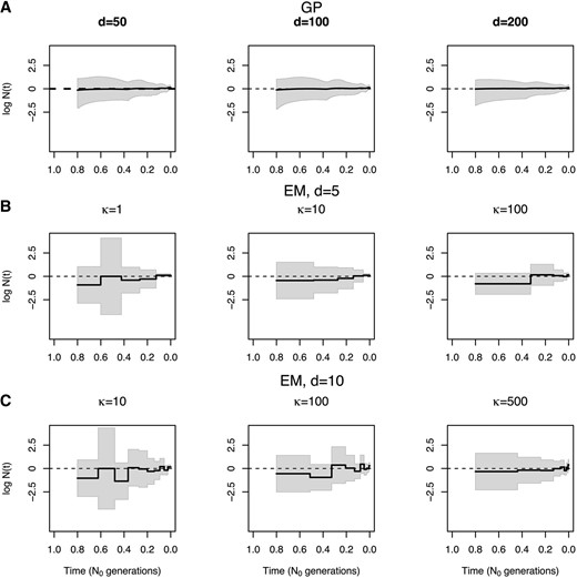
Sensitivity to parameter discretization. Population size trajectories estimated from one simulated genealogy () of 100 individuals with a constant population size are compared. We show true trajectories as dashed lines. (A) Bayesian GP estimates at and 200 equally spaced time points. (B) EM estimates of a piecewise constant trajectory with change points and and 100 (Equation 15). (C) EM estimates of a piecewise constant trajectory with change points and and 500 (Equation 15). Point estimates are shown as solid black lines. 95% percent credible intervals and 95% confidence intervals are shown by gray areas.
Summary statistics for simulation results depicted in Figure 4
| Simulation of a single genealogy with | SRE | MRW | ENV (%) |
|---|---|---|---|
| MLE | 41.80 | 14.76 | 100.0 |
| MLE | 41.05 | 2.98 | 100.0 |
| MLE | 57.12 | 1.72 | 100.0 |
| MLE | 47.93 | 16.08 | 100.0 |
| MLE | 61.77 | 3.91 | 100.0 |
| MLE | 31.52 | 3.60 | 100.0 |
| Bayesian GP | 6.98 | 1.88 | 100.0 |
| Bayesian GP | 5.52 | 2.15 | 100.0 |
| Bayesian GP | 4.96 | 1.70 | 100.0 |
SRE is the sum of relative errors (Equation 23), MRW is the mean relative width of the 95% BCI (Equation 24), and ENV is the envelope measure (Equation 25). Values in boldface type indicate best performance.
| Simulation of a single genealogy with | SRE | MRW | ENV (%) |
|---|---|---|---|
| MLE | 41.80 | 14.76 | 100.0 |
| MLE | 41.05 | 2.98 | 100.0 |
| MLE | 57.12 | 1.72 | 100.0 |
| MLE | 47.93 | 16.08 | 100.0 |
| MLE | 61.77 | 3.91 | 100.0 |
| MLE | 31.52 | 3.60 | 100.0 |
| Bayesian GP | 6.98 | 1.88 | 100.0 |
| Bayesian GP | 5.52 | 2.15 | 100.0 |
| Bayesian GP | 4.96 | 1.70 | 100.0 |
SRE is the sum of relative errors (Equation 23), MRW is the mean relative width of the 95% BCI (Equation 24), and ENV is the envelope measure (Equation 25). Values in boldface type indicate best performance.
Comparing methods for estimating
Figure 5 shows the estimated population size trajectories when the number of samples is two for the three different demographic scenarios and varying the number of local genealogies (100, 500, and 1000 local genealogies). For constant and exponential growth, our EM method assumes a piecewise constant trajectory of 10 change points () and using Equation 15 (similar to Li and Durbin 2011 and Rasmussen et al. 2014). For the bottleneck scenario, some of the intervals did not have coalescent events; hence, for this case we assumed a piecewise constant trajectory of 5 change points () and for constructing our EM estimates. We show the boxplots of the time to the most recent common ancestor (TMRCA) at the bottom of each plot in Figure 5, which indicate the uncertainty expected in our estimates.
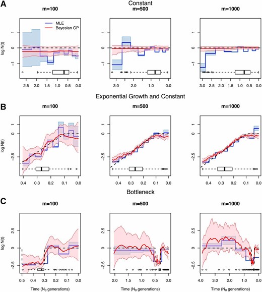
Inference of population size trajectories for a pair of individuals (). Simulated data under constant population size (A), exponential and constant trajectory (B), and a bottleneck (C). We show estimates from and local genealogies. Dashed lines show the true trajectories, blue lines and light blue areas represent EM point estimates and 95% confidence areas, and red lines and pink areas represent Bayesian GP posterior medians and 95% BCIs. Boxplots of the TMRCA are shown at the bottom of each plot.
Both approaches, EM and Bayesian GP, show narrower confidence and credible intervals at the center of the distribution of the TMRCA, particularly during the bottleneck in Figure 5C.
For the constant population size model in Figure 5A, our Bayesian GP considerably outperforms our EM estimates. This is not surprising since a priori has mean 0 in our Bayesian approach (Equation 16). Moreover, EM confidence intervals cover the truth only ∼30% of the time, while the GP method covers 100% of the truth (Table 4A). Despite placing a mean-0 prior on the Bayesian GP method accurately recovers sudden changes as shown in the bottleneck scenario. Although our Bayesian GP prior on is Brownian motion (which is not differentiable at any point), our Bayesian GP recovers smooth curves (Figure 5B).
Summary of simulation results depicted in Figure 5
| A. Simulations with n = 2 | |||||||||
|---|---|---|---|---|---|---|---|---|---|
| SRE | MRW | ENV | |||||||
| Simulation and method | m = 100 | m = 500 | m = 1000 | m = 100 | m = 500 | m = 1000 | m = 100 (%) | m = 500 (%) | m = 1000 (%) |
| Const. EM | 39.80 | 41.78 | 38.60 | 0.98 | 0.26 | 0.08 | 31.3 | 28.0 | 19.3 |
| Const. GP | 30.60 | 4.25 | 3.04 | 0.49 | 0.33 | 0.22 | 100.0 | 100.0 | 100.0 |
| Exp. EM | 64.68 | 25.70 | 33.70 | 0.91 | 0.16 | 0.12 | 42.0 | 26.0 | 6.6 |
| Exp. GP | 28.38 | 32.70 | 26.76 | 2.04 | 0.45 | 0.33 | 100.0 | 56.0 | 50.6 |
| Bottle. EM | 48.48 | 46.51 | 127.70 | 0.43 | 0.45 | 1.37 | 40.6 | 30.0 | 34.0 |
| Bottle. GP | 33.76 | 45.14 | 223.58 | 3.44 | 6.84 | 17.13 | 98.0 | 94.6 | 94.6 |
| B. Simulations with n = 20 | |||||||||
| SRE | MRW | ENV | |||||||
| m = 1 | m = 100 | m = 1000 | m = 1 | m = 100 | m = 1000 | m = 1 (%) | m = 100 (%) | m = 1000 (%) | |
| Const. EM | 60.87 | 121.30 | 25.60 | 2.28 | 2.16 | 0.23 | 100.0 | 37.7 | 39.3 |
| Const. GP | 31.74 | 3.94 | 13.22 | 1.06 | 0.70 | 0.36 | 100.0 | 100.0 | 100.0 |
| Exp. EM | 40.97 | 40.66 | 40.22 | 3.11 | 0.37 | 0.19 | 100.0 | 38.6 | 19.3 |
| Exp. GP | 25.35 | 27.03 | 65.61 | 3.53 | 1.56 | 0.42 | 100.0 | 100.0 | 39.3 |
| Bottle. EM | 147.93 | 78.40 | 78.20 | 6.98 | 0.81 | 68.4 | 66.0 | 78.6 | 49.33 |
| Bottle. GP | 68.93 | 78.2 | 50.92 | 2.74 | 2.47 | 1.47 | 92.0 | 79.3 | 78.6 |
| C. Simulations with n = 100 | |||||||||
| SRE | MRW | ENV | |||||||
| m = 1 | m = 100 | m = 1000 | m = 1 | m = 100 | m = 1000 | m = 1 (%) | m = 100 (%) | m = 1000 (%) | |
| Const. EM | 41.05 | 220.85 | 43.41 | 2.98 | 4.93 | 0.99 | 100.0 | 35.3 | 48.0 |
| Const. GP | 5.52 | 34.78 | 12.17 | 2.15 | 1.49 | 0.47 | 100.0 | 100.0 | 89.3 |
| Exp. EM | 76.86 | 40.22 | 27.63 | 3.23 | 0.81 | 0.13 | 87.3 | 42.0 | 14.0 |
| Exp. GP | 114.53 | 25.82 | 26.42 | 3.57 | 1.55 | 0.83 | 100.0 | 100.0 | 100.0 |
| Bottle. EM | 194.77 | 59.54 | 127.68 | 3.95 | 1.08 | 0.85 | 84.0 | 51.3 | 45.3 |
| Bottle. GP | 90.27 | 44.14 | 42.68 | 6.98 | 2.62 | 1.74 | 100.0 | 94.7 | 96.0 |
SRE is the sum of relative errors calculated as in (23), MRW is the mean relative width of the 95% BCI as Const: Constant population simulation scenario. Exp: Exponential growth followed by constant population size simulation scenario and Bottle: Population bottleneck. defined in (24), and ENV is the envelope measure calculated as in (25). Values in boldface type indicate best performance for each demographic model and sample size.
| A. Simulations with n = 2 | |||||||||
|---|---|---|---|---|---|---|---|---|---|
| SRE | MRW | ENV | |||||||
| Simulation and method | m = 100 | m = 500 | m = 1000 | m = 100 | m = 500 | m = 1000 | m = 100 (%) | m = 500 (%) | m = 1000 (%) |
| Const. EM | 39.80 | 41.78 | 38.60 | 0.98 | 0.26 | 0.08 | 31.3 | 28.0 | 19.3 |
| Const. GP | 30.60 | 4.25 | 3.04 | 0.49 | 0.33 | 0.22 | 100.0 | 100.0 | 100.0 |
| Exp. EM | 64.68 | 25.70 | 33.70 | 0.91 | 0.16 | 0.12 | 42.0 | 26.0 | 6.6 |
| Exp. GP | 28.38 | 32.70 | 26.76 | 2.04 | 0.45 | 0.33 | 100.0 | 56.0 | 50.6 |
| Bottle. EM | 48.48 | 46.51 | 127.70 | 0.43 | 0.45 | 1.37 | 40.6 | 30.0 | 34.0 |
| Bottle. GP | 33.76 | 45.14 | 223.58 | 3.44 | 6.84 | 17.13 | 98.0 | 94.6 | 94.6 |
| B. Simulations with n = 20 | |||||||||
| SRE | MRW | ENV | |||||||
| m = 1 | m = 100 | m = 1000 | m = 1 | m = 100 | m = 1000 | m = 1 (%) | m = 100 (%) | m = 1000 (%) | |
| Const. EM | 60.87 | 121.30 | 25.60 | 2.28 | 2.16 | 0.23 | 100.0 | 37.7 | 39.3 |
| Const. GP | 31.74 | 3.94 | 13.22 | 1.06 | 0.70 | 0.36 | 100.0 | 100.0 | 100.0 |
| Exp. EM | 40.97 | 40.66 | 40.22 | 3.11 | 0.37 | 0.19 | 100.0 | 38.6 | 19.3 |
| Exp. GP | 25.35 | 27.03 | 65.61 | 3.53 | 1.56 | 0.42 | 100.0 | 100.0 | 39.3 |
| Bottle. EM | 147.93 | 78.40 | 78.20 | 6.98 | 0.81 | 68.4 | 66.0 | 78.6 | 49.33 |
| Bottle. GP | 68.93 | 78.2 | 50.92 | 2.74 | 2.47 | 1.47 | 92.0 | 79.3 | 78.6 |
| C. Simulations with n = 100 | |||||||||
| SRE | MRW | ENV | |||||||
| m = 1 | m = 100 | m = 1000 | m = 1 | m = 100 | m = 1000 | m = 1 (%) | m = 100 (%) | m = 1000 (%) | |
| Const. EM | 41.05 | 220.85 | 43.41 | 2.98 | 4.93 | 0.99 | 100.0 | 35.3 | 48.0 |
| Const. GP | 5.52 | 34.78 | 12.17 | 2.15 | 1.49 | 0.47 | 100.0 | 100.0 | 89.3 |
| Exp. EM | 76.86 | 40.22 | 27.63 | 3.23 | 0.81 | 0.13 | 87.3 | 42.0 | 14.0 |
| Exp. GP | 114.53 | 25.82 | 26.42 | 3.57 | 1.55 | 0.83 | 100.0 | 100.0 | 100.0 |
| Bottle. EM | 194.77 | 59.54 | 127.68 | 3.95 | 1.08 | 0.85 | 84.0 | 51.3 | 45.3 |
| Bottle. GP | 90.27 | 44.14 | 42.68 | 6.98 | 2.62 | 1.74 | 100.0 | 94.7 | 96.0 |
SRE is the sum of relative errors calculated as in (23), MRW is the mean relative width of the 95% BCI as Const: Constant population simulation scenario. Exp: Exponential growth followed by constant population size simulation scenario and Bottle: Population bottleneck. defined in (24), and ENV is the envelope measure calculated as in (25). Values in boldface type indicate best performance for each demographic model and sample size.
Table 4A shows the performance statistics for the estimates of in Figure 5. In general, our Bayesian GP has wider credible intervals than the EM confidence intervals but these credible intervals cover the true trajectory better than the EM confidence intervals in all cases (MRW and ENV in Table 4). Our Bayesian GP estimates also generally have smaller sums of relative errors (SRE in Table 4). Under the bottleneck scenario, our Bayesian GP produces greater sums of relative errors than does the EM, but our Bayesian GP estimates recover the truth more accurately than the EM during the bottleneck.
Figure 6 and Figure 7 show our estimates when and (Table 4, B and C, gives performance statistics). In general, our GP-based estimates have smaller SRE and larger ENV than the EM-based estimates and hence, the MRW is usually wider in the GP-based estimates, accurately reflecting the uncertainty of the estimates. As expected, increasing the number of loci (m) generally decreases the width of the confidence and credible intervals of our estimates (MRW). Although this is generally true for EM estimates as well, EM estimates have very low coverage of the truth (MRE in Table 4) when the number of loci increases.
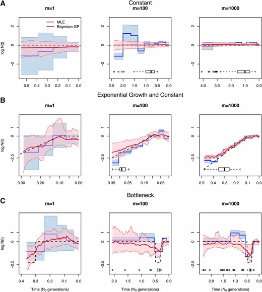
Inference of population size trajectories for Simulated data under constant population size (A), exponential and constant trajectory (B), and a bottleneck (C). We show estimates from genealogy, local genealogies, and local genealogies. Dashed lines show the true trajectories, blue lines and light blue areas represent EM point estimates and 95% confidence areas, and red lines and pink areas represent Bayesian GP posterior medians and 95% BCIs. Boxplots of the TMRCA are shown at the bottom of each plot.
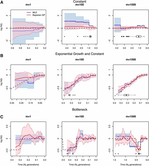
Inference of population size trajectories for Simulated data under constant population size (A), exponential and constant trajectory (B), and bottleneck (C). We show estimates from genealogy, local genealogies, and local genealogies. Dashed lines show the true trajectories, blue lines and light blue areas represent EM point estimates and 95% confidence areas, and red lines and pink areas represent Bayesian GP posterior medians and 95% BCIs. Boxplots of the TMRCA are shown at the bottom of each plot.
Sampling more individuals vs. sequencing more loci
Figure 5, Figure 6, and Figure 7 show our estimates for and 100 sampled individuals across varying numbers of loci. Performance of EM estimates depends strongly on the definition of the grid, so we focus here on the Bayesian GP estimates. We find that increasing the number of loci decreases uncertainty of our estimates and allows us to infer farther back in time. Increasing the number of samples does not necessarily increase the performance of our GP estimates (File S6). For example, under the bottleneck scenario, we are able to detect the bottleneck fairly accurately even for two samples with local genealogies. This is because most TMRCAs observed under the bottleneck scenario occur during the bottleneck (Figure 5, Figure 6, and Figure 7), regardless of the sample size. In contrast, in our exponential growth scenario, increasing the number of samples from to improves accuracy: point estimates are closer to the truth (SRE in Table 4, A–C) and credible intervals cover the truth completely (ENV of ).
Sequential Tajima’s genealogies are sufficient statistics under the SMC′
We defined transition densities in terms of coalescent times and quantities (see Methods: SMC′ calculations). The set of all quantities from a local genealogy forms a triangular matrix: an F matrix. We show that (i) F matrices are in bijection with ranked tree shapes and (ii) the set of local Tajima’s genealogies has sufficient statistics for inferring under the SMC′ model (see Appendix). These observations are crucial for inferring from sequence data directly. Coalescent-based inference from sequence data relies on marginalization over the hidden state space of genealogies. In the Appendix, we show that the state space needed is the space of local Tajima’s genealogies, as opposed to the space of local Kingman’s genealogies. For sequences, there are possible labeled topologies while only possible ranked tree shapes.
Application to human data
We applied our method to a 2-Mb region on chromosome 1 (187,500,000–189,500,000) with no genes from five Yorubans from Ibadan, Nigeria (YRI) and five Utah residents of central European descent (CEU) from the 1000 Genomes pilot project (1000 Genomes Project Consortium 2012) and previously analyzed for the same purpose (Sheehan et al. 2013). We used ARGweaver (Rasmussen et al. 2014) to obtain a sample path of local genealogies for the two populations (YRI and CEU). The parameters used were 200 change points, a mutation rate of and a recombination rate of (Rasmussen et al. 2014) (File S5). We note that ARGweaver assumes the SMC process and our method assumes the SMC′ process. Moreover, our inference is based on a single sample of the SMC process with known pruning times. Our ARGweaver set of local genealogies is discretized at 200 time points and our GP-based inference is influenced by this discretization. In Figure 8 we show our estimates of past Yoruban (in blue) and European population sizes (in green). The two population size trajectories experience a series of bottlenecks and overlap until ∼100 KYA, assuming a diploid reference population size of = 10,000 and a generation time of 25 years. In Figure 8 we recover an out-of-Africa bottleneck that starts ∼100 KYA and ends ∼30 KYA in the European population. These results are consistent with previously published results (Gronau et al. 2011; Li and Durbin 2011; Rasmussen et al. 2011; Sheehan et al. 2013; Schiffels and Durbin 2014). In File S5, Figure S4A, we show the estimates of instead of and time measured in units of generations (as in Figure 5, Figure 6, and Figure 7). We note that this two-step procedure of inferring local genealogies with ARGweaver and then using our method introduces biases and ignores genealogical uncertainty. In File S5, we correct for some of the bias caused by using this two-step procedure and show that our inferred population size trajectory remains valid for the recent past.
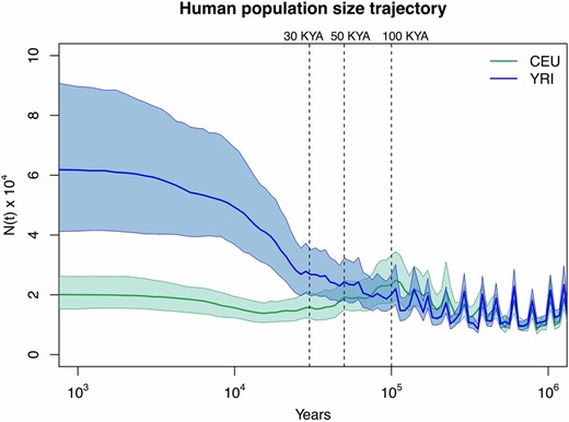
Inference of human population size trajectories for Green solid line and green areas represent the posterior median and 95% BCI for the European population (CEU) and blue solid line and blue areas represent the posterior median and 95% BCI for the Yoruban population (YRI). Time is measured in years in the past, assuming a generation length of 25 years and a reference diploid population of 10,000 individuals. The x-axis is log transformed.
Assessing the effect of using genealogies inferred with ARGweaver
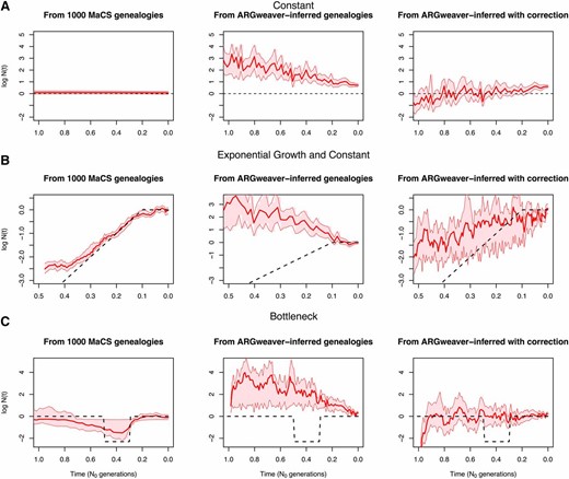
Assessing the effect of a two-step inferential approach. (A–C) Left, our GP-based estimates when 1000 local genealogies are known; center, our GP-based estimates when ARGweaver estimated local genealogies are used for inference; right, our corrected GP-based estimates when ARGweaver estimated local genealogies are used for inference.
Discussion
In this article, we propose a Gaussian-process-based Bayesian nonparametric method for estimating effective population size trajectories from a sequence of local genealogies, accounting for recombination. Under a variety of simulated demographic scenarios and sampling designs, our method recovers the truth with better precision and accuracy than a maximum-likelihood approach (Figure 5, Figure 6, and Figure 7). We apply our method to genealogies estimated using ARGweaver (Rasmussen et al. 2014) for European and African samples in the 1000 Genomes; this application to real data recovers the known features of the out-of-Africa bottleneck (Figure 8).
Several recent approaches have emerged for inferring population size trajectories from multiple whole-genome sequences using the SMC (Li and Durbin 2011; Sheehan et al. 2013; Schiffels and Durbin 2014). However, current SMC-based methods rely on maximum-likelihood inference (EM) of both a discretized parameter space and a discretized state space to gain computational tractability, and incur the costs of reduced accuracy and biased estimates. Although in principle the EM approach and the Bayesian nonparametric approach approximate similarly—by either a piecewise constant or a piecewise linear function—the Bayesian nonparametric approach is not affected by increasing the number of parameters (or change points) in the estimation of . For comparison with existing methods, we implemented an EM approach to infer population size trajectories from a sequence of local genealogies and we note that increasing the number of loci may actually increase the bias of the EM estimates (Figure 5, Figure 6, and Figure 7). For example, in simulation, our EM approach incorrectly detects the initial period of the simulated bottleneck ( instead of generations ago) with narrow confidence intervals (Figure 7C).
Using Bayesian GP for inferring population size trajectories offers many advantages over the EM approach. Similar to Palacios and Minin’s (2013) approach to inference from a single genealogy, we a priori assume that follows a log Brownian motion process. This allows us to model as a continuous positive function. The main advantage of using a Brownian motion process is that its inverse covariance function is a sparse matrix that allows for fast computations. Since the likelihood function involves integration over this integral is approximated by the Riemann sum over a regular grid of points. The finer the grid is, the better the approximation. We find that our method performs well for inferring at 100 change points in all our examples and, more importantly, results are not sensitive to the number of change points used in the analysis (Figure 4). Our Bayesian approach relies on MCMC for inference from the posterior distribution of model parameters. Because population sizes at different grid points are correlated, we adapt the recently developed MCMC technique splitHMC for jointly sampling all model parameters (Shahbaba et al. 2014; Lan et al. 2015). splitHMC is a Metropolis sampling algorithm that efficiently proposes states that are distant from current states with high acceptance rates. It has been shown to be more efficient in inferring from a single genealogy than elliptical slice sampling or regular Hamiltonian Monte Carlo sampling (Lan et al. 2015). However, splitHMC relies on calculating the score function at every single iteration. Because the pruning time in each local genealogy is unknown, we calculate the score function via Fisher’s formula.
In simulations, we find that our algorithm scales well with hundreds of individuals; our computational bottleneck is in the number of local genealogies. We envision that extending the current methodology to inference from sequence data directly will require a strategy for sampling shorter genomic segments. This would be a probabilistic alternative to arbitrarily choosing segment lengths (Sheehan et al. 2013; Rasmussen et al. 2014).
Under the SMC model, every recombination event along the genome translates to a new coalescent event for the sample under study, so increasing the number of loci results in more realizations of the coalescent process. The longer the segments are and the larger the number of samples taken, the greater the chance of observing variation due to recombination. This fact makes it hard to define a sampling strategy: Longer genomes or larger sample sizes? We show that increasing the number of local genealogies improves precision of our Bayesian GP estimates (Figure 5, Figure 6, and Figure 7). However, resolution into the past from contemporaneous sequences highly depends on the actual population size trajectory .
We used ARGweaver (Rasmussen et al. 2014) to generate two samples of contiguous local genealogies corresponding to a 2-Mb region of chromosome 1 for five Europeans (CEU) and five Africans (YRI) from the 1000 Genomes Project; this genomic region is free of genes and was also analyzed in Sheehan et al. (2013). Taking these two samples of local genealogies as our data (4186 local genealogies for CEU and 6247 local genealogies for YRI), we were able to use our Bayesian GP method to infer Yoruban and European effective population size trajectories (Figure 8). We find an out-of-Africa bottleneck that began ∼100 KYA and ended ∼30 KYA in the European population, consistent with Li and Durbin (2011); Rasmussen et al. (2011); Gronau et al. (2011); Sheehan et al. (2013), and Schiffels and Durbin (2014). We note that our estimates are based on a single sample of local genealogies and thus ignore genealogical uncertainty. Moreover, we generated our data from the posterior distribution of local genealogies, using ARGweaver at 200 time intervals, so our GP-based approach cannot fully detect sudden changes that may occur between the discretized times. In addition, ARGweaver assumes an SMC prior model on local genealogies and our GP-based method assumes the SMC′ process; the lack of invisible recombination events in ARGweaver’s genealogies will bias inference (as shown in simulated data in Figure 9).
The natural next extension for our method presented in this study is to infer from sequence data directly and not from the set of local genealogies. Our MCMC approach allows us to extend the current methodology in a Bayesian hierarchical framework where the SMC′ process would be used as a prior distribution over local genealogies. The work we present here suggests a combination of ARGweaver accommodating SMC′ and GP priors would result in an efficient method for inferring population size trajectories from sequence data directly. In addition, our model can be easily modified to model a variable recombination rate along chromosomal segments and to jointly infer variable recombination rates and .
Finally, we show that, under the SMC′ model, local ranked tree shapes and coalescent times correspond to a set of local Tajima’s genealogies; these Tajima’s genealogies are sufficient statistics for inferring . Under the SMC′ model, the state space needed for inferring population size trajectories from sequence data is that of a sequence of local Tajima’s genealogies. This lumping, or reduction of the original SMC′ process, will allow more efficient inference from sequence data directly.
Current methods for inferring population size trajectories make trade-offs to analyze whole genomes that limit both biological understanding of sudden population size changes and the ability to test hypotheses regarding population size changes. This work represents a critical set of theoretical results that lay the groundwork for efficient estimation of detailed histories from sequence data with measures of uncertainty.
Appendix
Discretization
For both our Bayesian method and our EM method, we assume that is a piecewise linear (or piecewise constant) function with d change points. Let be the ordered set of time points corresponding to the change points and the coalescent time points of local genealogy i. Then, we calculate all the factors needed for the observed data likelihood (Equation 13) and the complete data likelihood (Equation 19).
Expectation-Maximization Algorithm
E step
M step
Observed Score Function for Split Hamiltonian Monte Carlo
Our Bayesian approach relies on splitHMC sampling from the posterior distribution of model parameters. This method requires the calculation of the observed score function. We use Fisher’s identity and calculate the observed score function as the conditional expected complete score function. The lth element of is
Sufficient Statistics Under SMC′
Here, we first formally show that under the standard coalescent and for a single locus, the set of coalescent times has sufficient statistics for inferring that is, information about the topology is irrelevant for inference of . We then investigate the properties of our F quantities (see Methods: SMC′ Calculations) needed for the calculation of the transition densities (Equation 11) and show through a series of propositions that the F quantities and coalescent times are the sufficient statistics for inferring under the SMC′ process.
Proposition 1. For a single locus, the set of coalescent times are sufficient statistics for inferring .
Proof. This can be proved using the factorization theorem. The marginal density of a local genealogy (Equation 3) has a unique factor that depends on and g only through . The values of are induced by the natural order of the coalescent times.
▪
Let F denote a lower triangular matrix of size with the entry the number of lineages that do not coalesce in the time interval as defined in Methods: SMC′ Calculations and with the following properties:
for all (The first column contains 0’s for completion).
for all (lower triangular matrix).
for all (the diagonal corresponds to the number of lineages at each intercoalescent interval).
for all (at each intercoalescent interval, we lose two free lineages, so the second diagonal correspond to the number of lineages minus two).
- For the last row of F is defined according to
- Let c denote the number of cherries; then
For and if then
- Let denote the set of lineages in the intercoalescent interval with direct descendant internal nodes. The lineage labels correspond to the label of the coalescent time, when the direct descendant internal node was created. That is, the lineage created at has label n: the lineage created at has label i. Let denote the size of the set . Note that and
- For and if then at time there is a coalescence between a singleton and a lineage in the set . Let be the lineage selected uniformly at random from then
- For and if then at time there is a coalescence between two lineages and from the set . Let denote the minimum and the maximum of the two lineages selected; then
We show the correspondence between a ranked tree shape and the F matrix in the example of Figure A1. The first row and the first column are set to 0, and the first two diagonals are known with probability 1: and for In our example, and so the first diagonal corresponds to and the second diagonal corresponds to . The last row, contains 0, followed by the number of branches that do not coalesce in the time intervals and corresponding to .
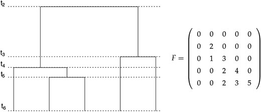
Ranked tree shape for
Proposition 2. There is a bijection between the set of ranked tree shapes and the set of F matrices.
▪
Note that the entries of the F matrix correspond to the same quantities needed to express the transition density of an invisible event (Equation 11). We claim that the sequence of coalescent times sets and matrices corresponding to the ranked tree shapes of local genealogies are sufficient statistics to infer under the SMC′ process. We prove this through Propositions 3–6.
Proposition 3. The probability density of Tajima’s genealogy is proportional, up to a combinatorial factor, to the probability density of Kingman’s genealogy.
Proposition 4. The marginal visible transition density from a local Kingman’s genealogy to is proportional to the marginal visible transition density from the corresponding local Tajima’s genealogy to .
▪
Proposition 5. The marginal invisible transition density from a local Kingman’s genealogy to is equal to the marginal invisible transition density from the corresponding local Tajima’s genealogy to .
▪
Proposition 6. The likelihood of partially observed embedded SMC ′ chain of local Kingman’s genealogies is proportional, up to a combinatorial factor, to the likelihood of partially observed embedded SMC ′ chain of the corresponding local Tajima’s genealogies.
Proof. The proof follows from Propositions 3–5 needed to express the likelihood of partially observed embedded SMC′ chain (Equation 13).
▪
Acknowledgments
We thank Amandine Veber for her valuable suggestions and comments. We thank Shiwei Lan for his suggestions for speeding up the MCMC sampling scheme and Sara Sheehan and Melissa J. Hubisz for helpful discussions. We also thank two referees for suggestions that improved this article. J.A.P. acknowledges scholarship from Consejo Nacional de Ciencia y Tecnología Mexico to pursue her research work. This research is supported in part by National Science Foundation CAREER award DBI-1452622 (to S.R.). S.R. is a Pew Scholar in the Biomedical Sciences, supported by The Pew Charitable Trusts, and an Alfred P. Sloan Research Fellow.
Footnotes
Communicating editor: Y. S. Song
Supporting information is available online at www.genetics.org/lookup/suppl/doi:10.1534/genetics.115.177980/-/DC1.
Literature Cited
Chen, W., 2011 Overlapping codon model, phylogenetic clustering, and alternative partial expectation conditional maximization algorithm. Ph.D. Thesis, Iowa State University, Ames, IA.
Griffiths, R. C., and P. Marjoram, 1997 An ancestral recombination graph, pp. 257–270 in Progress in Population Genetics and Human Evolution (IMA Volumes in Mathematics and Its Applications), Vol. 87, edited by P. Donnelly and S. Tavaré. Springer-Verlag, New York.
Murray, I., R. P. Adams, and D. J. C. MacKay, 2010 Elliptical slice sampling, Proceedings of the 13th International Conference on Artificial Intelligence and Statistics (AISTATS), Chia Laguna Resort, Sardinia, Italy, Vol. 9, pp. 541–548.
Neal, R. M., 2009 MCMC using Hamiltonian dynamics, pp. 113–162, edited by S. Brooks, A. Gelman, G. L. Jones, and X. -L. Meng. Hall, London/New York.
