


Abstract
Linkage disequilibrium is often measured by two statistics, D and r, which can be interpreted as the covariance and the correlation between loci and across gametes. When data consist of diploid genotypes, however, gametes cannot be identified. A variety of iterative statistical methods are used in such cases, all of which assume random mating. Previous work has shown that D and r can be expressed as covariances and correlations across diploid genotypes, provided that mating is random. We show here that this result also holds approximately when mating is nonrandom. This provides a means of estimating these parameters without iteration and without assuming random mating. This estimator is nearly as accurate as the widely used EM estimator and is many times faster.
IN diploid species, it is much easier to determine genotypes than haplotypes. Consequently, we are often ignorant about which nucleotides reside together on individual chromosomes. We are ignorant, in other words, about “gametic phase.” This makes it hard to measure statistical associations (“linkage disequilibrium,” LD) among loci. These associations are of interest for many reasons. They help us map disease loci, infer the histories of populations, and detect the effects of natural selection. The power of such studies has grown enormously as genome-scale databases, such as the HapMap (2007), have become available. On the other hand, their power is also limited by ambiguity about gametic phase.
The methods currently used to estimate LD (Hill 1974; Weir 1977; Excoffier and Slatkin 1995; Stephenset al. 2001) simplify the problem by assuming that populations mate at random. In most cases, some iterative algorithm is then used to converge gradually on a solution. In this article we introduce an approximate method that involves no iteration and allows for nonrandom mating. It is nearly as accurate as the widely used EM algorithm (Excoffier and Slatkin 1995) but much faster.
The approximation works with pairs of biallelic loci. In recent years, attention has shifted toward methods that reconstruct entire haplotypes involving many sites (Clark 1990; Excoffier and Slatkin 1995; Stephenset al. 2001). Yet pairwise methods remain important. They underlie several graphical methods in wide use (Dinget al. 2003; Barrettet al. 2005), they provide the backbone of descriptive studies of LD on genomic scales (HapMap 2005), they are used in mapping disease genes (Jorde 2000), and they are used to search for the effects of positive selection (Wanget al. 2006).
METHODS
Theory:
Several standard measures of LD can be expressed in terms of covariances across gametes. In this section, we derive analogous formulas in terms of covariances across diploid genotypes.
Eight parameters are needed to describe the complete distribution of genotypes at two biallelic loci (Weir 1996, pp. 125–127). We eliminate several of these dimensions by imposing the following constraints. First, we assume that PAB, PAb, PaB, and Pab have the same values among male and female gametes. This implies four constraints, three of which are independent. Another constraint involves the inbreeding coefficient, f—the probability that two homologous genes within a random individual are identical by descent (IBD). We assume that this probability is the same at each locus, thus imposing a fourth independent constraint. With these constraints, the original eight dimensions collapse to four. Thus, our model requires four parameters. We describe it in terms of pA, pB, f, and D.
We also introduce two sets of variables, one describing gametes and the other describing diploid individuals. For gametes, let y = 1 on A-bearing gametes and 0 on a-bearing gametes. Similarly, let z = 1 and 0 on B-bearing and b-bearing gametes. The means of y and z are pA and pB, and their variances are pA(1 − pA) and pB(1 − pB). For diploids, let Y = 2, 1, and 0 in genotypes AA, Aa, and aa, and let Z = 2, 1, and 0 in genotypes BB, Bb, and bb. Taking the two loci together, (yi, zi) represents the state of gamete i, where i = 1 or 2 within any diploid individual. Such an individual has state (Y, Z), where Y = y1 + y2 and Z = z1 + z2. If gametic phase is unknown, then we can observe Y and Z but not yi and zi. We refer to y and z as “genic values” and to Y and Z as “genotypic values.” It is well known that D is the covariance and r the correlation between y and z. In what follows, we introduce an approximation that extends these results to Y and Z.
We use the words “variance,” “covariance,” and “correlation” in two different ways: as functions of probability distributions and as functions of data. These words refer in the first sense to parameters and in the second to statistics. Where the meaning is not clear from context, we refer to “theoretical” or “sample” variances, covariances, and correlations.
In other words, the correlation between genotypic values is approximately equal to that between genic values.
Weir (2008) has derived similar formulas. Like us, he derives formulas for C(Y, Z). In the special case of random mating, he also shows that rYZ = r (Weir 2008, p. 132). Equation 5 suggests that Weir's result may be useful as an approximation even when mating is nonrandom.
These formulas suggest a simple way to estimate LD from unphased data. It is easy to estimate the sample correlation between genotypic values. Equation 5 implies that such estimates can be interpreted as estimates of r. These in turn can be transformed into estimates of D by inverting Equation 2. The statistical properties of these estimates are investigated below by computer simulation.
Computer simulations:
We used two types of computer simulation. The direct sampling algorithm (described in the appendix) specifies all parameter values, uses these to sample from the distribution of gametes, and then joins gametes to form diploid individuals. We use this approach to evaluate the approximation discussed above. This approach is flexible but requires arbitrary assumptions about the values of pA, pB, and r.
To avoid these arbitrary assumptions, we also examine the estimators using data generated by a coalescent simulation with recombination (Hudson 1990). In this simulation, the parameters we specify are those describing evolutionary history. We take the results of Schaffneret al. (2005) as a reasonable model of human evolutionary history, and their publication should be consulted for details. Briefly, their model holds that Europe and Asia were colonized from Africa, with bottlenecks at the time of colonization. Our program assumed random mating, a mutation rate of 2.2 × 10⁻⁸, and a recombination rate of 1 cm/Mb. It generated a simulated sample of 50 diploid “African” individuals, each with 1000 chromosomes. Chromosomes were 1 Mb long, and the average chromosome varied at 2979 polymorphic sites (SNPs) within the sample. Our program crawled along each chromosome, comparing each pair of SNPs within a moving 1600-SNP window, but excluding pairs >500 kb apart. Each comparison involved estimating r using the derived alleles at each of the two SNPs.
Both types of computer simulation generated samples of haploid gametes, which were used to calculate the “true value” of r2. True value is in quotation marks because there are really two versions of “truth”: (1) the value within the population as a whole and (2) the value within our sample of gametes with known phase. We measure deviations from the latter value because we are interested in the error resulting from unknown gametic phase.
Each simulation also combined gametes to form diploid genotypes with unknown gametic phase. The programs then used these data to estimate r2 by two methods: (1) the EM method introduced by Excoffier and Slatkin (1995) and (2) the method introduced here, which we refer to by our own initials (Rogers and Huff, RH). The EM algorithm is designed to reconstruct haplotypes involving many polymorphic loci. We coded a reduced version, which deals only with a pair of biallelic loci. This ensures that execution speed is not reduced by unnecessarily compex code. The EM algorithm works with a vector of haplotype frequencies, which it improves iteratively until some tolerance criterion is reached. Following Excoffier and Slatkin (1995), we set the tolerance parameter to 10−7. (In our version, this means that the sum of absolute differences between two successive frequency vectors is <10−7.)
RESULTS
The RH method is based on an approximation that is exact under complete linkage (c = 0) or when mating is random (f = 0). At larger values of c and f, approximation error generates bias, which should inflate the standard error (SE) of our estimates. For this reason, we expect SE to increase with c whenever f > 0. The larger the approximation error is, the steeper this rate of increase should be. Figure 1 uses this idea to evaluate approximation error. In Figure 1's top left panel, the curve for random mating (f = 0) appears to be completely flat, as expected in the absence of approximation error. In the other curves in that panel, f > 0 and error does increase with c, especially when inbreeding is strong. Yet even then, the approximation error is minor until c > 10−2. Even under strong inbreeding, therefore, the approximation is excellent for sites that are separated by <1 cM.
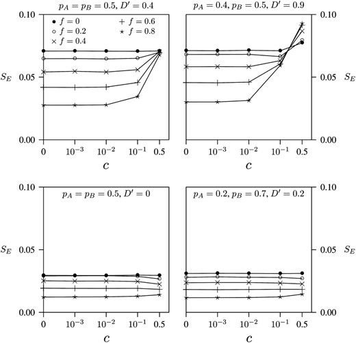
The effect of recombination rate (c) on the standard error (SE) of the RH estimator. Each point is based on 100,000 data sets simulated by direct sampling.
These conclusions depend on the particular values of pA, pB, and D′ that are assumed in the top left panel of Figure 1. The other panels of Figure 1 carry out the same analysis for different sets of parameter values. In the bottom two panels of Figure 1, D′ is near zero, and all of the curves are essentially flat, irrespective of the value of f. This suggests that there is little approximation error under weak LD, even if inbreeding is strong. This is consistent with our analytical error analysis (see above), in which the error was proportional to D. The top right panel of Figure 1 considers the case in which LD is very strong. In this case, strong inbreeding leads to a substantial approximation error, but as before this error is important only for loci separated by >1 cM. This is the only situation we have found in which the approximation error is large, and it refers to a situation—strong LD between essentially unlinked loci—that is unlikely to happen often in nature.
Each panel of Figure 1 also shows that SE declines with f. This makes sense because ambiguity about gametic phase arises from individuals who are heterozygous at both loci. In inbred samples, there are few such individuals and it is therefore easy to estimate LD (Fallin and Schork 2000).
The results just presented pertain to only one of the factors that contribute to statistical error. To study the others, we turn next to coalescent simulations. Figure 2 summarizes estimates of r2 based on 601,778,210 pairs of SNPs, which were generated by coalescent simulation. The EM method failed to converge in a small fraction (0.04%) of the comparisons. The pairs were sorted into 20 bins, on the basis of the physical distance separating the two SNPs. The left panel of Figure 2 shows the mean estimate of r2 within each bin. Both estimators show the expected pattern, with r2 declining as distance increases. X's indicate the means of the “true” values of r2. The means of both estimators are larger than the true values, indicating a small upward bias. This bias is a little larger for the RH method than for EM.
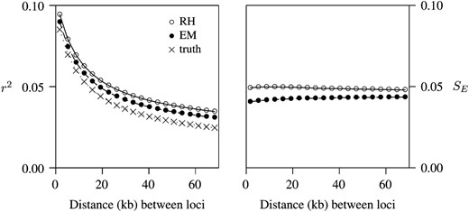
Performance of estimators of r2. Left, mean estimates of r2; right, standard errors (SE) of estimates.
The right panel of Figure 2 shows the standard errors (SE) of both estimators. (Note that these are the standard errors of individual estimates, not of the means displayed in the left panel.) The two estimators differ only a little. The EM algorithm has a small advantage (smaller SE), especially for tightly linked loci. For the RH estimator, the bias in estimates of r2 does not arise from any bias in the underlying estimates of r. On the contrary, these latter estimates are essentially unbiased (data not shown). Instead, the larger bias in the RH method reflects a larger sampling variance in estimates of r.
The smaller sampling variance of EM is not surprising, as EM is a maximum-likelihood estimator and should therefore have near-optimal statistical properties, at least in large samples. Nonetheless, this advantage appears to be small and should be weighed against other considerations.
One such consideration involves the assumption of random mating. EM makes this assumption, but the RH method does not. Consequently, one might suppose that inbreeding would introduce bias into EM estimates or elevate their standard errors. This, however, is not the case. As mentioned above, inbreeding makes it easier to estimate LD. Both estimators of r2 have smaller standard errors under inbreeding than under random mating. The bias and standard error of EM are consistently smaller than those of the RH method, even under inbreeding (data not shown).
Another consideration has to do with execution speed (Figure 3). Sample size affects the speed of both algorithms, but not in the same way. Both begin with the same initial step: a single pass through the data to construct a 3 × 3 table of genotype counts. Both algorithms then use this table in a second stage that does not depend on sample size. In the RH algorithm, this second stage is very fast, so the algorithm is dominated by the initial tabulation. Its execution time thus increases linearly with sample size. The second stage of the EM algorithm involves a series of iterations. This process is relatively costly and dominates when sample size is small. Execution time is thus insensitive to sample size except in large samples. In these larger samples, the tabulation step dominates, and execution time increases linearly with sample size. The RH algorithm is faster at all sample sizes, and this advantage is dramatic in small samples. With n = 25, for example, the RH algorithm is nine times as fast as EM. Even with n = 200, the RH algorithm is over twice as fast. These values refer to optimized C code, but a Python implementation exhibited similar behavior (data not shown).
![Execution times of estimators RH and EM. Each point is based on 100,000 function calls with f = 0, D′ = 0.4, and allele frequencies chosen at random on the interval [0.05, 0.95].](https://oup.silverchair-cdn.com/oup/backfile/Content_public/Journal/genetics/182/3/10.1534_genetics.108.093153/3/m_839fig3.jpeg?Expires=1716516862&Signature=jWYj-DPQkuQhpAOtuW87DL7pH~wbX6jOTQM9zMFqVNyL7-BU3Y7PJO8aOAiXAY3ThDphextQ88kBZeRysshMpIgf-dzMO7pFX1CCAOGzcTHn1skCdmjfFvjZ7BvXltNXdlVFDynyUhNzIphPvo7C6qxgUaNunQhrOqmY3QjhfC1mwZLKze6Iu2NkoezwMSGv~0pApvgMUbe6QA-G2MhS2BF6p-5l9G3~hLRRsTLnNyLuY4pQrVtcquee5zaVIT98nTeITcuKLBIY18XmtPse~WFVJAwuE7o3QYlAO7gtOCeGk7F3RAwDS3z-nBPLMEasLr~qufl2XDZsT4IPmVvUEg__&Key-Pair-Id=APKAIE5G5CRDK6RD3PGA)
Execution times of estimators RH and EM. Each point is based on 100,000 function calls with f = 0, D′ = 0.4, and allele frequencies chosen at random on the interval [0.05, 0.95].
DISCUSSION
The results reported here are based on approximate formulas that express LD in terms of covariances across diploid genotypes rather than across gametes. Equation 5 shows that r (the correlation across gametes) can be estimated from rYZ (the correlation across unphased genotypic values). From r it is easy to obtain other measures of two-locus LD, such as D or D′.
In this study, simulations were used to estimate the sampling distributions of all statistics. With real data, it would be easier to bootstrap across individuals or to use a randomization test. For example, one could randomly permute the genotypes at one of the two loci and then estimate D or r from the permuted data (Slatkin and Excoffier 1996). A thousand such estimates would approximate the sampling distribution of the statistic under the hypothesis of linkage equilibrium.
Our method involves several simplifying assumptions. First, it assumes that gamete types have equal frequencies within male and female gametes. Crow and Kimura (1970, pp. 44 and 45) discuss sex differences in allele frequencies, and their analysis also applies to gamete types. As they point out, these frequencies are ordinarily very similar in the two sexes but may differ in unusual circumstances. They might differ, for example, in a hybrid population in which males came from one population and females from another, or where most immigrants were of one sex, or where there was strong selection on one sex. Once these distorting influences end, however, the differences between male and female frequencies rapidly disappear. At an autosomal locus, they disappear in a single generation. Thus, the assumption of equal male and female frequencies should hold in most natural populations.
Our second assumption is about the probability (f) of identity by descent. This probability depends on the mating system and on population history, factors that might affect X, Y, and autosomal loci differently. Within any given chromosome, however, these factors should affect all neutral loci equally. Thus, f should have the same value at all neutral loci on any single chromosome. On the other hand, genotype frequencies may be distorted at individual loci either by selection or by genotyping errors. The RH method should be useful provided that these distorting influences are rare. These assumptions, of course, refer to the population rather than the sample. Even when our assumptions hold, estimates of f will vary from locus to locus because of the effects of sampling.
The EM estimator, which is currently in wide use, ignores the effect of inbreeding. The RH estimator, on the other hand, allows for inbreeding, but ignores recombination. Neither approximation seems to introduce appreciable error. Nonetheless, the bias and standard error of the RH estimator are somewhat larger than those of EM. This is not surprising, since EM is a maximum-likelihood estimator and inherits the near-optimal properties of that method. On the other hand, the RH estimator is much easier to code. It is so easy, in fact, that we now use it routinely in exercises assigned to an undergraduate population genetics class. In addition, the RH method is substantially faster—about nine times as fast as EM in samples of size 25. The current release of HapMap contains ∼4 million SNPs. To compare each of these with its neighbors within 1 Mb or so, one must make several billion comparisons. Thus, genome scans for LD involve a lot of computing, and the speed of the RH algorithm may be an important advantage.
Software for this project was written in Python, C, and Oracle. The Python and C programs are available at http://www.anthro.utah.edu/∼rogers/src/covld.tgz.
APPENDIX: DIRECT SAMPLING ALGORITHM FOR GENERATING DIPLOID GENOTYPES
In this probability distribution, gametes are classified by their state at the two loci. We also need to classify them in terms of identity by descent. In sexual species with separate sexes, homologous genes cannot be IBD from the generation of their parents. To avoid this issue, we model a population of monoecious sexuals. The inbreeding coefficient f represents the probability that two homologous genes are IBD from the generation of their parents.
A two-locus gamete is “recombinant” if an odd number of crossover events occurred between the two loci. This happens with probability c, the recombination rate. Within recombinant gametes, the two loci are independent provided that the parents mated at random. In comparing two-locus gametes, there are three cases to consider:
Case 1: Neither gamete is a recombinant, an event with probability (1 − c)2. In this case, the two gametes are IBD with probability f. Thus, we generate the first gamete by sampling from (A1). Then, with probability f, we duplicate the first gamete to obtain the second. Otherwise (with probability 1 − f), we sample once again from (A1).
Case 2: One gamete is a recombinant, an event with probability 2c(1 − c). In this case, the nonrecombinant gamete may be (i) IBD with the A/a locus of the recombinant (probability f), (ii) IBD with B/b (probability f), or (iii) IBD with neither locus (probability 1 − 2f). The nonrecombinant gamete cannot be IBD with both loci of the recombinant. To deal with these cases, our algorithm takes the following steps: (i) generate the nonrecombinant gamete by sampling from (A1); (ii) with probability f, obtain the A/a locus of the second gamete by copying the first; otherwise sample from Bernoulli(pA); and (iii) obtain the B/b locus of the second gamete in an analogous fashion.
Case 3: Both gametes are recombinants, an event with probability c2. At each locus, the two genes are IBD with independent probability f. In that case, the two genes at each locus are generated by independent samples from the appropriate Bernoulli distribution. Otherwise (with probability 1 − f), they are two copies of a single Bernoulli variate.
Footnotes
Communicating editor: L. Excoffier
Acknowledgements
We are grateful for comments from Henry Harpending, Lynn Jorde, Jon Seger, and Bruce Weir. Initial experiments with the RH algorithm were done by students in two of our classes, and we are grateful to them as well.
References
Clark, A. G.,
Crow, J. F., and M. Kimura,
Excoffier, L., and M. Slatkin,
Hudson, R. R.,
Lewontin, R. C., and K.-i. Kojima,
Wang, E. T., G. Kodama, P. Baldi and R. K. Moyzis,
Weir, B. S.,
Weir, B. S.,
