


Abstract
It is useful to detect allelic heterogeneity (AH), i.e., the presence of multiple causal SNPs in a locus, which, for example, may guide the development of new methods for fine mapping and determine how to interpret an appearing epistasis. In contrast to Mendelian traits, the existence and extent of AH for complex traits had been largely unknown until Hormozdiari et al. proposed a Bayesian method, called causal variants identification in associated regions (CAVIAR), and uncovered widespread AH in complex traits. However, there are several limitations with CAVIAR. First, it assumes a maximum number of causal SNPs in a locus, typically up to six, to save computing time; this assumption, as will be shown, may influence the outcome. Second, its computational time can be too demanding to be feasible since it examines all possible combinations of causal SNPs (under the assumed upper bound). Finally, it outputs a posterior probability of AH, which may be difficult to calibrate with a commonly used nominal significance level. Here, we introduce an intersection-union test (IUT) based on a joint/conditional regression model with all the SNPs in a locus to infer AH. We also propose two sequential IUT-based testing procedures to estimate the number of causal SNPs. Our proposed methods are applicable to not only individual-level genotypic and phenotypic data, but also genome-wide association study (GWAS) summary statistics. We provide numerical examples based on both simulated and real data, including large-scale schizophrenia (SCZ) and high-density lipoprotein (HDL) GWAS summary data sets, to demonstrate the effectiveness of the new methods. In particular, for both the SCZ and HDL data, our proposed IUT not only was faster, but also detected more AH loci than CAVIAR. Our proposed methods are expected to be useful in further uncovering the extent of AH in complex traits.
THERE has been growing interest in detecting causal variants in fine mapping for a disease or complex trait of interest, which can tell us about the biological mechanisms of the disease or trait. The most challenging part is to distinguish the true causal variants that biologically influence the trait and the variants that are only statistically associated due to linkage disequilibrium (LD) with the causal variants. A common approach is to use colocalization tests to infer whether a variant is causal for both the trait and a molecular intermediate trait like gene expression, through which the causal variant influences the trait. Many methods have been proposed for testing colocolization, but most of them assume there is no more than one causal variant in each locus. When multiple causal variants exist, those methods may lose their effectiveness. As a result, it is important to know whether multiple causal variants are in a locus and, if so, how many they are. The presence of multiple causal variants in a locus is called allelic heterogeneity (AH).
AH is known to be common for Mendelian traits, and it may also happen to common diseases and complex traits. In particular, its presence may influence the interpretation of some biological phenomena. For example, a previous study seemed to show that multiple epistatic effects affect gene expression (Hemani et al. 2014), which means that the effect of a variant on a trait is influenced by other variants elsewhere in the genome. However, according to Wood et al. (2014), most of those effects may be explained by a single third variant in that locus. This shows that the existence of AH or lack of it will critically determine whether there is an epistasis in a locus, and thus it is important to study AH.
One common approach to test AH is to use a so-called standard conditional analysis, in which one tests each SNP conditioning on the already detected significant SNPs (Yang et al. 2012). This conditional analysis operates as a sequential forward variable/SNP selection procedure, which is known to be unstable and nonoptimal in general. Hormozdiari et al. (2017) proposed an alternative method called CAVIAR (causal variants identification in associated regions) that was proven to outperform the standard conditional analysis in most cases. However, since CAVIAR calculates the posterior probabilities for all possible subsets of causal SNPs, its computing time can be very long when the number of SNPs is huge. Accordingly, it imposes an assumption on the maximum number of causal SNPs in a locus, say six, to save computing time. However, as will be shown, the assumed maximum number of causal SNPs will not only determine the computing time, but also influence the final result. Finally, as a Bayesian method, CAVIAR gives the posterior probability of AH; albeit useful, it may be difficult to calibrate a posterior probability with a commonly used statistical significance level. For example, as will be shown, CAVIAR’s recommended significance cut-off of a posterior probability at ≥ 0.9 (to declare AH) may be too conservative when compared to a usual nominal family-wise type I error rate.
Technically, testing AH is similar to testing pleiotropy, which means that a SNP influences more than one trait. A direct way to test pleiotropy is to conduct the intersection-union test (IUT), which was first mentioned by Schaid et al. (2016) and used by Deng and Pan (2017b). We propose a new hypothesis testing approach to test for AH, based on the IUT with a joint/conditional model and the Wald tests. Note that our conditional model is based on the full set of the SNPs in a locus, differing from the standard conditional analysis of Yang et al. (2012) that is based on sequential forward variable/SNP selection, which is known to be unstable and nonoptimal with the cost of multiple testing/selection. In contrast, our IUT is based on a full joint/conditional model on all SNPs, on which we test the null hypothesis of no AH directly, which is expected to be more powerful and stable than the sequential selection of SNPs. In particular, in the context of fine mapping, Benner et al. (2017) pointed out that the sequential approach to conditional analysis is inferior to that based on the full joint/conditional model as adopted in FINEMAP (a software package for efficient variable selection using summary data from genome-wide association studies) (Benner et al. 2016). After determining the presence of AH, we also propose two sequential testing procedures with IUT (Seq IUT) to infer the number of causal SNPs. We will demonstrate the effectiveness of our new approaches with simulated and real data, including large-scale schizophrenia (SCZ) and high-density lipoprotein (HDL) genome-wide association study (GWAS) summary data sets.
Methods
Testing AH
Our above formulation follows that of Schaid et al. (2016) in the context of testing pleiotropy. As a reviewer points out, since we have , we can construct the IUT by taking as its final P-value; that is, we do not have to use for . In theory, it is possible to have each , but not, rejected for , we feel that conceptually it is better to include to construct and thus the IUT, which might be slightly more conservative than otherwise.
Sequential testing
We propose a Seq IUT procedure to estimate the number of causal SNPs in the presence of AH, following the idea of Schaid et al. (2016). We can test : only elements of are nonzero using the same IUT approach. consists of (): the SNPs in J are causal, while the others are not. To test , the Wald test statistic is , where , are obtained from , after deleting the SNPs in J. Under the null, follows . Then, we can calculate the P-value for each smaller test and compare the minimum with . This IUT for looks at all the possible combinations of s causal SNPs and tests whether the remaining SNPs are all noncausal. If every combination is rejected, we can conclude that the number of causal SNPs is not equal to s. Since the number of possibilities may become too huge as s goes up, we also suggest setting a maximum number of causal SNPs k. The sequential testing procedure is:
Test (no causal SNPs) at level by comparing with . If we reject , go to the next step; otherwise stop and conclude the number of causal SNPs is 0.
Test , , ..., one by one with IUT until the first time that one of them is not rejected at level . If () is the first one that is not rejected, conclude the number of causal SNPs is m. If , , ..., are all rejected, conclude that the number of causal SNPs is bigger than k.
The type I error rate (i.e., the probability of rejecting the null hypothesis with the true number of causal SNPs) of this sequential test is controlled at level α as well. Suppose the true number of causal SNPs is m. If we only test at level α with its IUT, the rejection probability is α. In the sequential procedure, we need to test and reject all of them to reject , so the probability of rejecting is no greater than α, the rejection probability of only testing .
Since we need to consider all possibilities in each step of Seq IUT, it can be very slow when the number of SNPs is big. We propose a faster version of the procedure, called Seq IUT 2:
Test and in the same way as Seq IUT does. If both of them are rejected, test each SNP separately in the joint model and find the most significant one, denoted by .
Test with IUT; however, instead of considering all the possible combinations of two causal SNPs, only consider the ones including SNP , which is assumed to be significant already. There are only cases left. If is rejected by IUT, test each possible combination of causal SNPs in the joint model and find the most significant set, which is .
Test , assuming that and are significant and should always be included in the combinations of causal SNPs. This process is repeated until an insignificant result is obtained.
The difference between Seq IUT 2 and Seq IUT is that Seq IUT 2 keeps adding significant SNPs and thus is able to decrease the number of combinations that we need to consider. In this way, not only is Seq IUT 2 faster, but it can also tell us which SNPs are significant. The two sequential procedures are conceptually similar to usual sequential procedures used in variable selection except that here we are testing AH, instead of testing the significance of individual parameters or being based on a model selection criterion like AIC (Akaike information criterion)/BIC (Bayesian information criterion).
Data availability
The subset of the SCZ GWAS summary statistics (Schizophrenia Working Group of the Psychiatric Genomics Consortium 2014) with the 103 loci after SNP pruning as used in this paper is available at https://doi.org/10.6084/m9.figshare.6615461, while that of the HDL imputed GWAS summary statistics (Pasaniuc et al. 2014) with the loci being used in this paper is available at https://doi.org/10.6084/m9.figshare.6463292. The R packages “jointsum” and “AHIUT” can be downloaded from https://doi.org/10.6084/m9.figshare.6615482 and https://doi.org/10.6084/m9.figshare.6615470.
Results
Simulations
We conducted simulation studies that were similar to that of Hormozdiari et al. (2017). We looked at the 1000G (1000 Genomes) CEU (Northern Europeans from Utah) population (1000 Genomes Project Consortium et al. 2015) with 503 subjects and chose some genes on chromosome 1 that had at least one SNP associated with some trait in the National Human Genome Research Institute GWAS Catalog. For each gene, we deleted some SNPs to control all of the SNP pairwise correlations within 0.9. After excluding the loci with only one SNP, we ended up with 237 loci (genes) with eight SNPs on average in each locus. The range of the number of SNPs in a locus was 2–40.
Then, we simulated GWAS summary statistics with no epistasis interaction using the same approach as in Hormozdiari et al. (2017). Since we only needed the LD structure and effect sizes to simulate summary statistics in this scenario, we directly used the LD structure estimated from the 1000G data and assumed that was the correlation structure for simulated subjects. In each locus, there were one or two causal SNPs, which were randomly decided. The normalized effect size of a causal SNP, defined as where β is the effect size and σ is the SD of the error term, was chosen to be close to those in Hormozdiari et al. (2017). Denote the normalized effect size in a locus by . For a locus with one causal SNP, we assumed that the normalized effect size was for that SNP and 0 for the others. For a locus with two causal SNPs, the normalized effect size was and for those SNPs and 0 for the others. For instance, if the first and second SNPs in a locus are causal, the normalized effect size is . If the first and last SNPs are causal, , and so on. The summary statistics for that locus were simulated from .
After obtaining the summary statistics and the LD structure for each locus, we carried out CAVIAR and IUT to get the posterior probabilities and P-values, respectively. Then, we compared the true positive rates (power) and false positive rates (type I error) using receiver operating characteristic (ROC) curves. Note that for the IUT, when we estimated the joint model, we took as the marginal effect size and assumed that the SE was 1 and the sample size was 1000. We also directly used the LD structure estimated from the 1000G data. For CAVIAR, we set the maximum number of causal SNPs to six.
As shown in Figure 1, the performances of CAVIAR and IUT were close, though CAVIAR performed slightly better at extremely low false positive rates. Nevertheless, CAVIAR took much longer (at ∼90 sec per data set) to run than IUT (at ∼1 sec per data set). We can expect that if the number of SNPs is further increased, CAVIAR’s computation time will go up dramatically because it compares models per locus. Meanwhile, IUT will still be fast, since it only involves one model and Wald tests per locus. We also repeated the process to generate multiple data sets and applied the methods to all of them. The ROC curves did not change much.
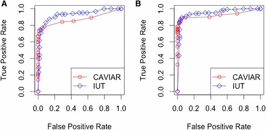
ROC curves for CAVIAR and IUT. (A) , . (B) , . CAVIAR, causal variants identification in associated regions; IUT, intersection-union test; ROC, receiver operating characteristic.
In another simulation, we compared the IUT and CAVIAR in terms of detecting the number of causal SNPs. For each locus containing > 12 SNPs, we assumed that there were one to three causal SNPs with the same effect size. We generated 10 data sets and applied the two approaches to calculate the true positive rates for different numbers of causal SNPs, defined as the proportion of the loci that were predicted correctly. We chose , the maximum number of causal SNPs, to be six for the methods.
The result is shown in Table 1. For Seq IUT, the number of causal SNPs was determined by when the sequential process stopped. For CAVIAR, the number of causal SNPs was the one with the highest posterior probability; (*) determined the number of causal SNPs by requiring its posterior probability to be ≥ 0.8.
True positive rates for predicting the number of causal SNPs ()
| CAVIAR (*) | Seq IUT (Seq IUT 2) | |||||
|---|---|---|---|---|---|---|
| No. causal SNPs | 1 | 2 | 3 | 1 | 2 | 3 |
| True positive rate | 0.92 (0.008) | 0.56 (0.016) | 0.25 (0.057) | 0.81 (0.81) | 0.49 (0.39) | 0.31 (0.30) |
| True negative rate | 0.58 | 0.39 | 0.26 | 0.59 (0.65) | 0.42 (0.43) | 0.35 (0.41) |
| Computation time (seconds) | 813 | 14 (13) | ||||
The computation time is for all loci. Normalized effect size = 4.89 or 0. CAVIAR, causal variants identification in associated regions; No., number of; Seq IUT, sequential intersection-union testing procedure.
| CAVIAR (*) | Seq IUT (Seq IUT 2) | |||||
|---|---|---|---|---|---|---|
| No. causal SNPs | 1 | 2 | 3 | 1 | 2 | 3 |
| True positive rate | 0.92 (0.008) | 0.56 (0.016) | 0.25 (0.057) | 0.81 (0.81) | 0.49 (0.39) | 0.31 (0.30) |
| True negative rate | 0.58 | 0.39 | 0.26 | 0.59 (0.65) | 0.42 (0.43) | 0.35 (0.41) |
| Computation time (seconds) | 813 | 14 (13) | ||||
The computation time is for all loci. Normalized effect size = 4.89 or 0. CAVIAR, causal variants identification in associated regions; No., number of; Seq IUT, sequential intersection-union testing procedure.
When the true number of causal SNPs was small, Seq IUT was much faster than CAVIAR, since it could come to an early stop instead of having to enumerate all possible combinations of causal SNPs. However, if the number of causal SNPs is larger, Seq IUT may lose its advantage, since it also needs to assess many possible combinations before it can stop. For instance, detecting 6 causal SNPs out of 40 SNPs using the for loop in R may take 8 min. Seq IUT 2 was faster than Seq IUT, and the speed advantage would be much larger as the number of SNPs went up. The result of Seq IUT 2 was also not much worse than that of Seq IUT.
SCZ data
To compare the performance of the methods on real data, we examined the reported 108 independent and significant loci in a SCZ GWAS (Schizophrenia Working Group of the Psychiatric Genomics Consortium 2014), which gives the GWAS summary statistics based on ∼150,000 subjects. We chose the SNPs in the exact range of each genomic region that was reported by the Schizophrenia Working Group of the Psychiatric Genomics Consortium (2014), and then removed some SNPs in each region to ensure that none of the pairwise absolute correlations between any two SNPs was > 0.9. Note that this procedure might be different from what was done by Hormozdiari et al. (2017), in which the data preprocessing procedure or definition of the significant loci was not provided. We ended up with 103 loci containing multiple SNPs. We calculated the Z-scores using the reported odds ratio estimates and the SE of log odds ratios, and then carried out the methods using the 1000G data as the reference panel (1000 Genomes Project Consortium et al. 2015). For CAVIAR, we chose based on , the number of SNPs in a locus. The number of SNPs in a locus ranged from 3 to 407, with an average of 86. While the cut-off for the posterior probability for AH was set to 0.8, as suggested by Hormozdiari et al. (2017), we tried two nominal significance levels for the IUT: one was based on a Bonferroni correction for testing the 103 loci, and the other was based on the usual genome-wide significance level (with a genome-wide scan).
As shown in Table 2, regardless of the significance level used, the IUT detected more significant loci than CAVIAIR, which was perhaps mostly due to the noncompatible significance cutoffs between the two approaches. For the 18 AH loci detected by IUT () but missed by CAVIAR (with larger k’s), the mean posterior probabilities of having one and two causal SNPs were 0.364 (with range: 0.211–0.608) and 0.369 (with range: 0.267–0.475), respectively; the mean posterior probability of AH was 0.635 (with range 0.387–0.789). For 10 out of the 18 loci, the number of causal SNPs being two yielded the highest posterior probability.
Numbers of significant loci with AH for SCZ
| CAVIAR | IUT | ||
|---|---|---|---|
| No. significant loci (overlap with CAVIAR) | 28/32 | 60 (27/31) | 49 (27/31) |
| Computation time (min) | 9.9/2022 | 6.5 | |
| CAVIAR | IUT | ||
|---|---|---|---|
| No. significant loci (overlap with CAVIAR) | 28/32 | 60 (27/31) | 49 (27/31) |
| Computation time (min) | 9.9/2022 | 6.5 | |
In each cell, “a/b” indicates the different results for cases A and B. Case A: when and otherwise. Case B: when and when . CAVIAR, causal variants identification in associated regions; No., number of; IUT, intersection-union test.
| CAVIAR | IUT | ||
|---|---|---|---|
| No. significant loci (overlap with CAVIAR) | 28/32 | 60 (27/31) | 49 (27/31) |
| Computation time (min) | 9.9/2022 | 6.5 | |
| CAVIAR | IUT | ||
|---|---|---|---|
| No. significant loci (overlap with CAVIAR) | 28/32 | 60 (27/31) | 49 (27/31) |
| Computation time (min) | 9.9/2022 | 6.5 | |
In each cell, “a/b” indicates the different results for cases A and B. Case A: when and otherwise. Case B: when and when . CAVIAR, causal variants identification in associated regions; No., number of; IUT, intersection-union test.
While CAVIAR became much slower as went up, using a larger led to more discoveries, demonstrating the importance of specifying a large k at the expense of possibly too long a computing time. The 32 significant AH loci identified by CAVIAR using larger values covered the 28 identified with smaller k values. The one AH locus that IUT did not cover was the same as shown in Figure 4, which will be discussed later. Note that our results from CAVIAR covered only some of the 25 loci reported in Hormozdiari et al. (2017), possibly due to different SNPs included in the loci. We also tried to define the loci by expanding from the lead SNPs and obtained similar results.
In Figure 2, for a locus with 38 SNPs, marginal analysis detected no significant SNPs among them, which means that the significant lead SNP was deleted in the pruning process. Meanwhile, the conditional analysis found multiple significant SNPs, three of which were highly significant. The IUT detected AH in this case (P-value = 2.7e−14) and the Seq IUT method inferred the number of causal SNPs as five. However, CAVIAR did not detect AH in this case (with a posterior probability of AH = 0.63 < 0.8). However, the posterior probabilities of having 0–2 causal SNPs were 0.0006, 0.37, and 0.47, respectively, with 0.47 being the highest among posterior probabilities of having 0–6 causal SNPs, so CAVIAR would infer that the number of causal SNPs was two. This may indicate that, for CAVIAR, the results of testing AH and finding the number of causal SNPs could be contradictory to each other.
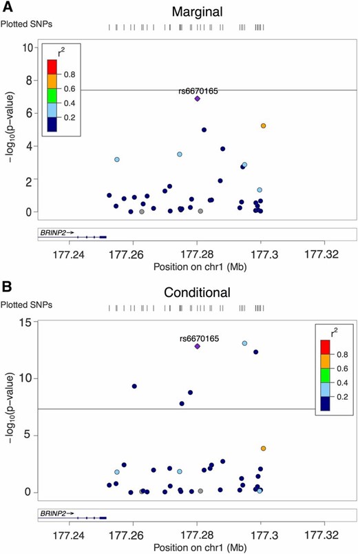
Allelic heterogeneity in one locus associated with schizophrenia. (A) LocusZoom plot of 38 SNPs’ P-values in marginal analysis. (B) LocusZoom plot of the same SNPs’ P-values in conditional analysis. Horizontal line: significance cut-off 5e−8. chr1, chromosome 1.
As shown in Figure 3, in another locus with 31 SNPs, the marginal analysis found three significant SNPs, while the conditional analysis did not detect any. IUT concluded that there was no AH, and Seq IUT inferred the number of causal SNPs as zero, which agreed with the conditional analysis result. With the posterior probability of AH being 0.56, CAVIAR did not declare AH either. However, like the previous case, CAVIAR suggested that the number of causal SNPs should be predicted as two, since its posterior probability was the highest (0.46).
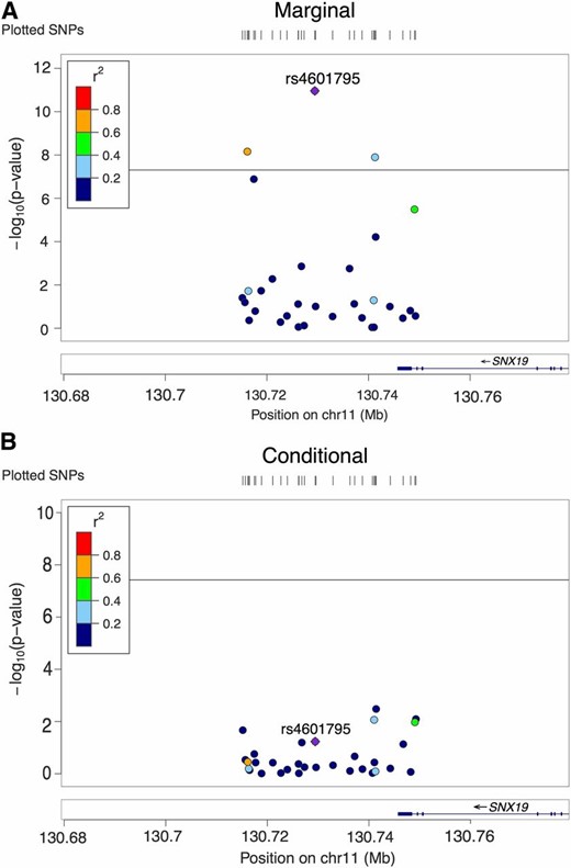
No allelic heterogeneity in one locus associated with schizophrenia. (A) LocusZoom plot of 31 SNPs’ P-values in marginal analysis. (B) LocusZoom plot of the same SNPs’ P-values in conditional analysis. Horizontal line: significance cut-off 5e−8. chr11, chromosome 11.
Figure 4 shows the only AH locus identified by CAVIAR but missed by IUT. The eigenvalues of the LD matrix for the SNPs in the locus ranged from 0.0018 to 10, suggesting that the LD matrix was not singular. CAVIAR inferred the number of causal SNPs as two, which were SNPs rs4936215 and rs695134; however, the conditional analysis said otherwise. The posterior probability of AH was 0.849, which was above the threshold of 0.8. The posterior probabilities of having 0–6 causal SNPs were 5.0e−7, 0.15, 0.46, 0.28, 0.087, 0.017, and 0.0025, respectively. In contrast, the P-value of the IUT for testing AH was 0.019. Note that when we used 0.05 as the cut-off for IUT and Seq IUT, they detected AH and found two causal SNPs (rs12294011 and rs145205826). The P-values of having one or less causal and two or less causal SNPs were 0.019 and 0.100, respectively. When we used the faster sequential approach with a cut-off of 0.05, it detected three causal SNPs (rs12294011, rs145205826, and rs79071988); the P-values of having one or less, two or less, and three or less causal SNPs were 0.019, 0.027, and 0.061, respectively. The P-values for rs4936215, rs695134, and rs10894771 in the full conditional model were 0.003, 0.08, and 0.91, respectively, with the P-value of their joint test being 0.0063, while that of testing rs4936215 and rs695134 was 0.0069. Furthermore, we also tried forward sequential selection of significant SNPs one by one, which was the conditional method mentioned in Hormozdiari et al. (2017): in the first six steps, the six most significant SNPs (and their P-value) were: rs4936215 (8.2e−11), rs695134 (1.3e−3), rs12294011 (8.3e−3), rs4936214 (3.8e−3), rs35261319 (0.014), and rs145205826 (0.0502). Hence, we conclude no strong evidence to support AH as reported by IUT.
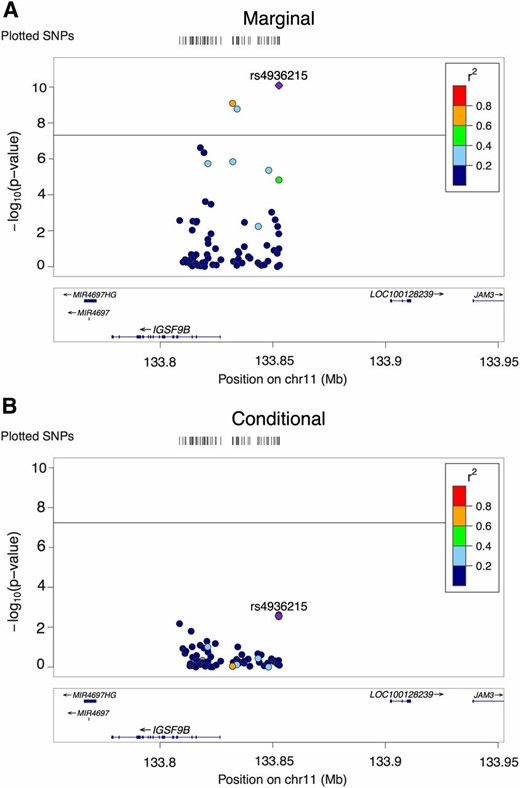
One locus associated with schizophrenia. (A) LocusZoom plot of 68 SNPs’ P-values in marginal analysis. (B) LocusZoom plot of the same SNPs’ P-values in conditional analysis. Horizontal lines: significance cut-off 5e−8. chr11, chromosome 11.
HDL data
We also applied the methods to the summary statistics for HDL, imputed and provided by Pasaniuc et al. (2014). We focused on the 43 genes reported to contain SNPs associated with HDL in Teslovich et al. (2010) and used the 1000G reference again. The procedure was almost the same as that in the previous section for SCZ data. Each locus included the SNPs within 500 kb of the lead SNP. If any of the included significant SNPs (P-value < 5e−8) were 500 kbp upstream or downstream and correlated to the lead SNP (), they were expanded by 500 kbp in both directions as well. Before conducting the analyses, we deleted some SNPs to make sure that none of the correlations were > 0.9 or < −0.9, while keeping the lead SNPs. When the LD matrix was nearly singular even after pruning, we took the generalized inverse of a matrix when needed, instead of the (ordinary) inverse, to avoid the numerical issue. However, when the number of SNPs was high, it was still possible to end up with a poor covariance matrix estimate for the regression coefficient estimates with some negative diagonal elements. In this case, we applied a simple regularization method by adding a small constant (0.01) to the diagonal of the LD matrix and then dividing the whole matrix by 1.01 (to ensure its positivity).
In this case, IUT again detected no fewer significant AH loci than CAVIAR did, as shown in Table 3. The significant loci detected by CAVIAR covered 12 of the 13 significant loci reported by Hormozdiari et al. (2017). The difference was most likely due to different definitions of the loci. IUT became much slower as the number of SNPs became too high, because of its implementation in R (with its inefficiency of for loops and of inverting large matrices). For instance, with SNPs, the computation time of IUT was ∼4.3 hr, which could be improved by a implementation in a high-level language like C, as for CAVIAR. The two loci detected by CAVIAR but not IUT were the same for different choices of .
Numbers of significant AH loci for HDL
| CAVIAR | IUT | ||
|---|---|---|---|
| No. significant loci (overlap with CAVIAR) | 30/34 | 35 (28/32) | 34 (28/32) |
| Computation time (hr) | 0.3/42.4 | 9.4 | |
| CAVIAR | IUT | ||
|---|---|---|---|
| No. significant loci (overlap with CAVIAR) | 30/34 | 35 (28/32) | 34 (28/32) |
| Computation time (hr) | 0.3/42.4 | 9.4 | |
In each cell, “a/b” indicates the different results for cases A and B. Case A: when ; when ; and otherwise. Case B: when ; when ; when ; and otherwise. CAVIAR, causal variants identification in associated regions; No., number of; IUT, intersection-union test.
| CAVIAR | IUT | ||
|---|---|---|---|
| No. significant loci (overlap with CAVIAR) | 30/34 | 35 (28/32) | 34 (28/32) |
| Computation time (hr) | 0.3/42.4 | 9.4 | |
| CAVIAR | IUT | ||
|---|---|---|---|
| No. significant loci (overlap with CAVIAR) | 30/34 | 35 (28/32) | 34 (28/32) |
| Computation time (hr) | 0.3/42.4 | 9.4 | |
In each cell, “a/b” indicates the different results for cases A and B. Case A: when ; when ; and otherwise. Case B: when ; when ; when ; and otherwise. CAVIAR, causal variants identification in associated regions; No., number of; IUT, intersection-union test.
Discussion
Here, we have presented IUT for testing for AH, as well as Seq IUT and Seq IUT 2, two sequential testing procedures to infer the number of causal SNPs in the presence of AH. Our simulation results showed that the performance of IUT in terms of ROC was similar to that of CAVIAR, while the speed of IUT could be much faster, especially when the number of SNPs was not too small and not too big. After applying the methods to the large-scale SCZ and HDL GWAS summary data, we found more significant loci with AH using IUT than using CAVIAR with much less computational time. In addition, to save computing time in CAVIAR, one has to specify a relatively small number, k, of maximum causal SNPs for each locus; when applied to the SCZ and HLD data, we found that specifying too large a k could take too much time, but at the same time, using a smaller k led to the detection of a smaller number of AH loci by CAVIAR. We note that our statistical model for the joint distribution of the summary statistics in a locus is the essentially the same as that of CAVIAR. For predicting the number of causal SNPs, our proposed Seq IUT performed similarly to CAVIAR in the simulations, but it is expected to be faster, more so when the true number of causal SNPs is much smaller than the assumed maximum number of causal SNPs. The faster version, Seq IUT 2, further saves time, and its performance was no worse than that of Seq IUT in the simulations. The current speed advantage of our IUT-based methods over CAVIAR is expected to be more dramatic if we implement them in Rcpp (or a high-level language like C as for CAVIAR). Finally, we note that our statistical model for the joint distribution of the summary statistics in a locus (as a multivariate normal distribution) is the essentially the same as that of CAVIAR. The main difference is that we separate the problem of testing AH from that of estimating the number of causal SNPs; the former is much faster than the latter, which requires some time-consuming exhaustive or sequential searching.
Acknowledgments
This research was supported by National Institutes of Health grants R01 GM-113250, R01 GM-126002, R01 HL-105397, R01 HL-116720, and R21 AG-057038, by National Science Foundation grant DMS 1711226, and by the Minnesota Supercomputing Institute at the University of Minnesota.
Footnotes
Supplemental material available at Figshare: https://doi.org/10.6084/m9.figshare.6463292.
Communicating editor: G. Churchill
Literature Cited
Berger, R. L., 1997 Likelihood ratio tests and intersection-union tests, pp. 225–237 in Advances in Statistical Decision Theory and Applications, edited by S. Panchapakesan and N. Balakrishnan. Birkhäuser, Boston.
