


Abstract
The purpose of this chapter in FlyBook is to acquaint the reader with the Drosophila genome and the ways in which it can be altered by mutation. Much of what follows will be familiar to the experienced Fly Pusher but hopefully will be useful to those just entering the field and are thus unfamiliar with the genome, the history of how it has been and can be altered, and the consequences of those alterations. I will begin with the structure, content, and organization of the genome, followed by the kinds of structural alterations (karyotypic aberrations), how they affect the behavior of chromosomes in meiotic cell division, and how that behavior can be used. Finally, screens for mutations as they have been performed will be discussed. There are several excellent sources of detailed information on Drosophila husbandry and screening that are recommended for those interested in further expanding their familiarity with Drosophila as a research tool and model organism. These are a book by Ralph Greenspan and a review article by John Roote and Andreas Prokop, which should be required reading for any new student entering a fly lab for the first time.
The Genome
THE basic karyotype of Drosophila melanogaster, which can be seen in mitotically active neuroblasts of the larval brain, is comprised by four chromosomes, the X and Y sex chromosomes, two larger autosomal elements, chromosomes 2 and 3, and the small dot fourth chromosome (Figure 1) (Metz 1914; Deng et al. 2007) . The X is also referred to as the First chromosome and designated with a “1.” In naming and symbolizing chromosome aberrations, the numeral is commonly used rather than the letter when the sex chromosome is involved. Females have two X chromosomes and males a single X and the Y. Both sexes have two sets of the autosomal second, third, and fourth chromosomes. The X is divided into two arms by the position of centromere, a large left arm (XL) and a much smaller right arm (XR), and is thus acrocentric. The Y is also acrocentric with a slightly longer long arm (YL) and a short arm (YS). The two larger autosomal chromosomes are metacentric with the centromere residing in the center of two roughly equal left and right arms. The fourth dot chromosome is acrocentric, similar to the X. The small arm is designated as left (4L) and the larger as right (4R). In sum, there are a total of 10 chromosome arms: XL, XR, YL, YS, 2L, 2R, 3L, 3R, 4L, and 4R. The reason for the X, 2, 3, and 4 arms being designated left and right while the Y is designated long and short is clouded by the mists of time.
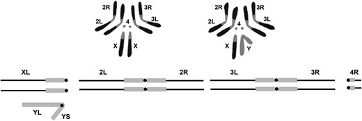
The upper portion of the figure shows a representation of the karyotype of D. melanogaster. Chromosomes from female third instar larval neuroblasts on the left and males on the right. Below is a diagrammatic representation of the genome indicating the names of the arms of the sex chromosomes and autosomes. Note that the small XR and 4L arms are not shown. The euchromatic portions of the genome are shown in black and the heterochromatin in gray.
It is also possible to characterize the chromosomal complement by the distribution of the heterochromatic and euchromatic portions of the genome. In this case heterochromatin, is defined as that portion of the karyotype that stains more darkly and is more compact in standard preparations. It is also late replicating in S phase of the cell cycle, is the residence of highly repeated DNA sequences, and is enriched in intermediate repeat naturally occurring transposable elements (Dimitri 1997). The regions of the X, second, and third chromosomes adjacent to the centromeres are darkly staining and are referred to as the pericentric heterochromatin. The Y and fourth are also darkly staining and appear entirely heterochromatic in neuroblast preparations; however, the fourth does have a small euchromatic right arm (Figure 1).
Using a series of differential staining techniques (quinacrine, Hoechst, and N and C banding) it has been possible to cytologically subdivide the pericentric heterochromatin and the Y chromosome (Gatti et al. 1976; Pimpinelli et al. 1976). Heterochromatin was initially considered to be genetically inert and devoid of genes. This has been shown to be incorrect, and while gene density in these regions of the genome is low there are indeed bona fide genes (Gatti and Pimpinelli 1992; Dimitri et al. 2003, 2009). The heterochromatic regions are seen as brightly fluorescent blocks separated by less darkly-stained regions and constrictions. Starting with the telomere of YL these regions are numbered sequentially (YL = 1–17, YS = 18–26; XL = 26–31, XR = 32–34; 2L = 35–38, 2R = 39–46; 3L = 47–52, 3R = 53–58; and 4L = 59–61) (Figure 2). Blocks 20 on the X and 29 on the Y correspond to the positions of the Nucleolus Organizer, the site of the tandemly repeated ribosomal RNA genes on the sex chromosomes.
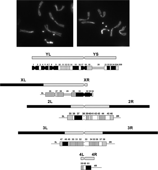
Photomicrographic and diagrammatic representation of the heterochromatic elements of D. melanogaster. The photomicrographs show male larval neuroblasts stained with Hoechst. The brightly fluorescent dots are the fourth chromosome and the longer bright chromosome the Y. The diagram below shows the position of the pericentric heterochromatin of the X, second, and third chromosomes, and the Y and fourth. Below each heterochromatic region, the differentially-staining blocks of these regions of the chromosomes are shown. The position of the centromere is indicated by a constriction. Modified from Gatti and Pimpinelli (1992).
One of the best characterized of these genomic components is the Y chromosome. The Y is unnecessary for viability but XO males lacking this chromosome are sterile. Additionally, XXY animals are female, thus the Y has no role in sex determination (sex is determined by the X autosome balance: X:A = 1 is ♀ and X:A = 0.5 is ♂). Early genetic analyses of the Y demonstrated that male fertility requires six fertility factors, four mapping to YL and two to YS (Brosseau 1960). This initial study was extended by using a set of chromosome aberrations that deleted or otherwise disrupted the linear continuity of the Y. These aberrations were then cytologically mapped and characterized with respect to their effects on male fertility (Kennison 1981; Hazelrigg et al. 1982; Gatti and Pimpinelli 1983). The results demonstrated that the positions of the fertility factors were spread along the arms of the Y and were associated with the less densely stained small constrictions between the brightly fluorescent blocks (Figure 3). Subsequent molecular mapping of the Y demonstrated that, in addition to the genetically identified fertility factors, there are at least five additional protein-coding genes on the Y (de Carvalho et al. 2000, 2001; Vibranovski et al. 2008).
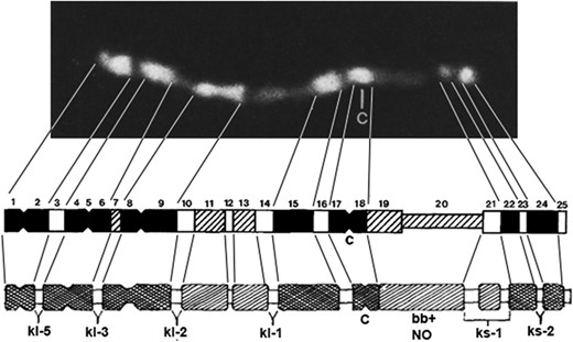
Cytogenetic map of the Y chromosome of D. melanogaster. At the top is a photomicrograph of the banding pattern of a Hoechst-stained Y chromosome. Below are diagrammatic representations of the banding revealed by differential staining of the Y. The darker blocks correspond to more brightly-staining regions. The position of the centromere is indicated by a constriction and the letter c. Genetic mapping has positioned the YL (kl-5, kl-3, kl-2, and kl-1) and YS (ks-1 and ks-2) male fertility factors in the dim regions adjacent to the bright blocks. The bobbed locus or nucleolus organizer region (ribosomal RNA cistrons) is in YS between the bright blocks at the centromere and the distal pair at the telomere of the short arm.
Similar analyses have been done for the pericentric heterochromatin of the two large autosomes. Using a variety of chromosomal aberrations and differential staining techniques, mutations that result in discernable defects (e.g., lethality) have been mapped to these regions (Dimitri 1991; Koryakov et al. 2002; Rossi et al. 2007; Coulthard et al. 2010; He et al. 2012; Figure 4). Here again, molecular mapping in these same regions has revealed additional protein coding loci that are clearly expressed but have not been identified by mutations. The genes located in both the Y and the pericentric heterochromatin tend to be quite large relative to those in the euchromatic regions of the genome. The transcription units of the protein coding genes tend to be made up of normal coding exons separated by large intronic regions that contain multiple copies of transposable elements (de Carvalho et al. 2003).
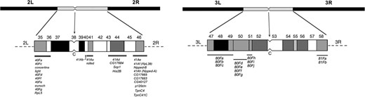
Diagrams of heterochromatic blocks of chromosomes 2 and 3 and the positions of the genes located in the pericentric heterochromatin. The position of the centromere is indicated by a constriction and the letter C. The blocks are numbered as in Figure 2. The position of the genes is shown by bars below the block diagrams and the list of the genes below the bars. The brightly fluorescing blocks are black, less bright in gray and dull regions in white. After Dimitri et al. (2009).
The Polytene Chromosomes
The cytogenetic mapping of the heterochromatin, while informative, admittedly lacks resolution. This resolving power is enormously enhanced by the presence of the polytene chromosomes. Their discovery in the early days of Drosophila research provided what can be viewed as an initial high-resolution view of the genome and a first foray into the genomics of a higher eukaryote. These chromosomes are found in several cell types, the function of which is principally secretory. In Drosophila, the most useful are found in the larval salivary glands. These cells undergo several rounds of endoreduplication in which S phase is repeated with no subsequent mitosis. In the case of the third larval instar, the ploidy level reaches 1024 (Rodman 1967; Hammond and Laird 1985). This level of ploidy is reached by the euchromatic portions of the genome while the heterochromatin is vastly underreplicated. Another feature peculiar to Drosophila is the fact that chromosomes show what is referred to as somatic pairing. As in meiosis, homologous regions of the chromosome tend to associate. The combined effect of polyploidy and pairing is that the 1024 DNA strands for each euchromatic chromosome arm form a coherent coil, and one can observe five large arms corresponding to X, 2L, 2R, 3L, and 3R. The small 4R can be seen as well. All of these arms emanate from a central region called the chromocenter. This is the residence of the pericentric heterochromatin and, in the case of males, the Y chromosome. The chromosomes are large enough that they are easily seen using standard light microscopy. Each of the euchromatic arms has a unique banding pattern caused by differential condensation of the chromatin into darkly-staining bands and less dense interbands. In actual fact, staining is not absolutely necessary to see the banding patterns of the arms since they are clearly resolved using phase contrast illumination.
Like the differential staining of the heterochromatic blocks, the banding pattern of the polytene chromosomes has been codified to provide mapping coordinates (Bridges 1935; Figure 5). The pattern is that each large arm is divided into 20 roughly equal numbered segments (X = 1–20; 2L = 21–40; 2R = 41–60; 3L= 61–80; 3R = 81–100; and the small fourth 4R = 101–102). The numbered segments each begin with a darkly-staining prominent band. Each of these numbered units is subdivided into six roughly equal lettered segments, A–F, and the bands in each lettered segment are numbered. Using this coordinate system, each band has a unique name and its position is discernible from that name. Band 3C2 is on the X chromosome near the telomere while 77B3 is near the base of chromosome 3L (Figure 5). The original maps produced and shown in Figure 5 were hand-drawn camera lucida images (Bridges 1935). These drawings were subsequently improved upon by the production of a set of lovely photographic montage maps (Figure 6) (Lefevre 1976). Additionally, the chromosomes have been embedded and sectioned for TEM analyses and the banding pattern revealed at high resolution (Saura et al. 1997, 1999). Interestingly, the banding patterns figured in the original Bridges maps were not markedly altered by this later analysis. Until the sequencing of the genome and the production of annotated molecular maps, these drawn and photographic maps were the lingua franca when discussing genetic mapping of genes to the genome. The chromosome aberrations discussed below can be easily resolved in polytene chromosome preparations, and when these changes in genome structure are associated with genetic loci the latter can be mapped with reasonable precision.
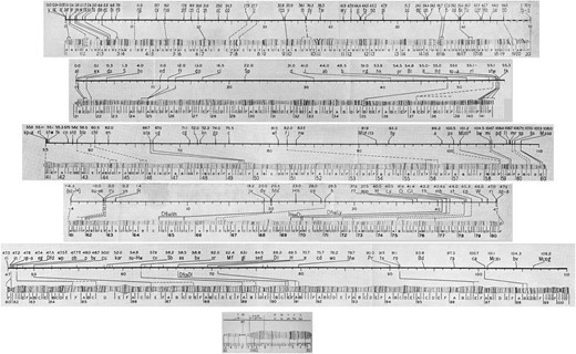
The original polytene chromosome map drawings of Bridges (1935). The band pattern names are shown below the drawings and are described in the text. The lines above the chromosomes show the recombination map positions (numbers below the lines) and the genes with their individual map positions above the lines. Those genes which had been localized cytologically to the chromosomes are joined to the chromosomes by solid and dotted lines connecting the position of the gene on the recombination map to the bands of the polytene chromosomes.
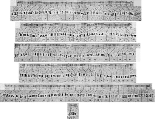
The photographic polytene chromosome maps of Lefevre (1976). These maps are collages of idealized segments of the polytene chromosomes. Below each arm are the positions of the numbered segments using Bridges’ nomenclature. Above each arm are the corresponding drawing taken from Bridges’ original maps. The bands demarking each numbered segment are connected by lines between each of the two map versions.
The Molecular Genome
A watershed moment in the history and utility of flies occurred when the consortium of the Berkeley Drosophila Genome Project and Celera Genomics produced a sequence and assembly of the D. melanogaster genome (Adams et al. 2000; Myers et al. 2000). In this initial iteration of the assembly most of the gene models were ab initio predictions. In the years since the original publication the annotation of the genome has been improved enormously, notably by the inclusion of data from global RNA sequencing analyses used to inform on the validity of gene models coupled with the inclusion of large regions of heterochromatin to the bases of the major euchromatic arms and the Y chromosome (modENCODE et al. 2010; Cherbas et al. 2011; Graveley et al. 2011; Boley et al. 2014; Brown et al. 2014; Chen et al. 2014). In the last few updates of the genome produced by FlyBase there has been little churn and few changes in the annotations of the molecularly-mapped genes. The genome has matured into one of the best characterized among the metazoans. The following description is taken from the FB2016_05 (R6.13) release version of the genome (http://flybase.org).
At that release, the total sequence length is 143,726,002 bp with a total gap length, including major and minor scaffolds, of 1,152,978 bp [Table 1 (shows only the major scaffolds)]. Most of the gaps are in the heterochromatin. The sequence is assembled into 1870 scaffolds with the majority of sequence, 137.6 Mbp, residing on the seven chromosome arms (X, Y, 2L, 2R, 3L, 3R, and 4) plus the entire mitochondrial genome (Table 1). The sequence includes contiguous portions of the pericentric heterochromatin of X, 2, 3, and 4. There are 1862 “unlocalized” minor scaffolds, of which 884 have been mapped cytologically or genetically to the heterochromatic portions of: X, 2CEN, 3CEN, Y, and XY. Some can also be mapped to the highly repeated rRNA-encoding genes found in the nucleolus organizer (NO) of the X and Y (He et al. 2012).
Size in nucleotides of the sequenced and annotated genome of D. melanogaster FB2016_05 (R6.13)
| Scaffold | Length (bp) | Sized Gaps | Total Gap Size (bp) in Scaffold | Unsized Gaps |
|---|---|---|---|---|
| X | 23,542,271 | 4 | 65,520 | 6 |
| 2L | 23,513,712 | 0 | 0 | 2 |
| 2R | 25,286,936 | 1 | 6,000 | 7 |
| 3L | 28,110,227 | 4 | 117,660 | 5 |
| 3R | 32,079,331 | 9 | 22,772 | 18 |
| 4 | 1,348,131 | 1 | 17,000 | 0 |
| Y | 3,667,352 | 61 | 242,633 | 150 |
| M | 19,524 | 0 | 0 | 0 |
Annotation of the genome identifies 17,728 genes, of which 13,907 are protein coding, and these encode 21,953 unique polypeptides. The remaining 3821 identified loci are various types of RNA noncoding genes (Table 2). It is unlikely that there will be a significant amount of change in the number of protein coding genes, albeit some is possible. However, the genes in the nonprotein coding set could change more dramatically as this class of loci gains more attention and further characterization takes place.
Listing of the coding and noncoding gene types and their number in D. melanogaster FB2016_05 (R6.13)
| Gene Type | Number |
|---|---|
| Protein coding | 13,907 |
| rRNA | 147 |
| tRNA | 313 |
| snRNA | 31 |
| snoRNA | 288 |
| miRNA | 256 |
| LncRNA | 2,470 |
| Pseudogenes | 315 |
| Gene Type | Number |
|---|---|
| Protein coding | 13,907 |
| rRNA | 147 |
| tRNA | 313 |
| snRNA | 31 |
| snoRNA | 288 |
| miRNA | 256 |
| LncRNA | 2,470 |
| Pseudogenes | 315 |
| Gene Type | Number |
|---|---|
| Protein coding | 13,907 |
| rRNA | 147 |
| tRNA | 313 |
| snRNA | 31 |
| snoRNA | 288 |
| miRNA | 256 |
| LncRNA | 2,470 |
| Pseudogenes | 315 |
| Gene Type | Number |
|---|---|
| Protein coding | 13,907 |
| rRNA | 147 |
| tRNA | 313 |
| snRNA | 31 |
| snoRNA | 288 |
| miRNA | 256 |
| LncRNA | 2,470 |
| Pseudogenes | 315 |
How Many Genes Are There?
As noted above, there are 17,728 genes annotated in the molecular genome. A total of 3622 of these have an associated mutant allele. Thus, the functional significance of a majority of the molecularly defined loci apart from an assumed role based on sequence identity remains to be determined. This latter point is coupled with the statistic that there are 14,348 mutant alleles that identify “genes” but these have not been mapped to the molecular genome. Are the 14,348 identified mutants assignable to the 17,728 or is the relationship more complicated? The answer is of course: “It’s more complicated.”
Some light can be thrown on the answer by looking at studies that have attempted to saturate specific small regions of the genome with mutations. As an example, I will use one of my favorites, the zeste (z) – white (w) interval on the X chromosome (Figure 7). The z locus maps to 3A3 with molecular coordinates X:2,447,769.2,450,550; w is at 3C2 molecular coordinates X:2,790,599.2,796,466. Thus, between the two genes there is a 340,049 bp length of DNA that is home to 42 identified and annotated transcription units, two of which are pseudogenes. Saturation of this interval with mutations has revealed the presence of 13 loci that mutate to lethality, two to sterility, and one to periodic behavior (Judd et al. 1972; Lim and Snyder 1974; Young and Judd 1978). Of the 13 lethals, nine have been mapped to the genome; the other four have yet to be molecularly mapped but presumably each is associated with one of the remaining transcripts. The sterility and period genes have also been associated with specific transcription units. This leaves 19 molecularly mapped loci that are either immutable or that classical methods cannot ascribe a clear functional role to, and at least one that is indispensable to the fly. The z-w interval is not unique. Saturation studies carried out throughout the genome repeatedly provide a similar result; there are molecularly identified genes that are conserved across the genus that do not appear to be necessary for a viable, fertile adult fly and these loci could make up half or more of the genome. Like the cosmologists, we apparently have genomic dark matter.
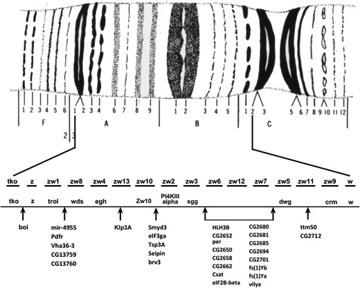
Genetic saturation map of the zeste – white interval on the X chromosome. The banding pattern of the 3A1,2–3C2,3 is shown at the top. Using zeste in 3A2 and white in 3C2 as left and right positions, this interval contains 14 polytene bands on Bridges’ map. The first line below the map shows the names and order of the lethal loci identified in saturation screens. The next line shows the positions and identity of genes mapped at the molecular level, which are known alleles of the original genetically identified lethals. The lists below are genes known from the molecular annotation of this interval with arrows indicating their positions relative to the genetic map. Note that there are many more molecularly defined loci than have genetically identified lesions. In addition to the loci listed in this figure, there are ∼30 additional mutations provisionally assigned to this interval whose allelic relationship to either the molecularly or genetically identified loci has yet to be determined. After Judd et al. (1972).
Moving forward, a goal of genetic analyses in Drosophila will be to determine the molecular identity of the 14,348 unmapped mutations and, more of an enigma, the functional significance of the “dark matter.”
Changes in Chromosome Structure
As noted above, the polytene chromosomes have allowed the ready determination of large-scale changes in chromosome structure both within and between members of the karyotype. The smallest of these are deficiencies and duplications of segments of the chromosome arms. The more straightforward of the two are the deficiencies, which are simply deletions of contiguous regions of the genome. These are named according to the chromosome and arm affected. Thus, a deficiency on the fourth chromosome is Df(4) with a unique identifier following the closing parenthesis. Examples of the deletion domains of Dfs localized to the sequence of the fourth chromosome are shown in Figure 8. Deficiencies that can be identified cytologically have been used to localize genes to specific regions of the genome, and those with known molecular endpoints can be used to define the genomic interval in which a gene resides. They have also been extremely useful in studies designed to saturate small regions of the genome similar to the z-w example noted above. In many cases, the endpoints of deficiencies have been localized to the genomic sequence and, as noted if this is known, the deficiency serves to place the exposed gene in a defined region of the genome. Several hundred of such deficiencies have been assembled in the stock collection at the Bloomington Drosophila Stock Center (BDSC, http://flystocks.bio.indiana.edu) and have become a valuable resource for localizing mutations to the genome.
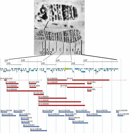
Diagrammatic representation of the extent of deletions and duplications molecularly mapped to the fourth chromosome. At the top are photographic and drawing maps of the chromosome with the Bridges’ numerical and lettered subdivisions indicated below the drawing. Lines extending from the map show the corresponding intervals on the molecular map. The blue arrows below the map intervals show the position and direction of transcription of the loci annotated to the sequence of the chromosome. The red bars below the loci indicate the position and extent of the deficiencies. The blue bars beneath the deficiencies indicate the position and extent of the segregating duplications, which have been made by transgenic fragments. After Lefevre (1976) and FlyBase.
Duplications are a bit more complicated in the sense that they can be of different types depending on the number of chromosome arms involved. The simplest type is the tandem duplication, designated, for example, Dp(2;2) followed by a unique identifier. The duplicated region can be either direct ABC:ABC or reversed ABC:CBA. This type of duplication tends to be unstable, especially the tandem reversed repeat, due to the fact that pairing and exchange can take place within the duplicated region resulting in resolution of the repeat into a single sequence. Duplications can also occur within or between chromosome arms but not be tandem. These are still given a similar designation, e.g., Dp(3;3)##. Finally, there are the segregating duplications. These are characterized by the transposition of a genomic fragment from one chromosome to another and are designated by, for example, Dp(2;3) or Dp(1;Y), again followed by a unique identifier. The numbers and/or letters in the parenthesis indicate the chromosome elements involved, with the first number or letter indicating the origin of the duplication and the second the new position. The duplicated material can either be inserted into or be appended to the recipient chromosome. In Figure 8 the positions of a series of Dp(4;3) are shown. These are transgenically created, cloned genomic fragments that have been inserted into a third chromosome landing site by the ϕC31 integrase system (Groth et al. 2004). A like set of Dp(2;3) that tile and cover the X chromosome has also been created (Venken et al. 2010). A systematic study using more traditional methods has also been used to create a series of larger X chromosome duplications that are appended to the Y chromosome. Again, these duplications have known molecular endpoints and can be mapped both cytologically and molecularly (Cook et al. 2010). Segregating duplications of the X chromosome are particularly valuable for the genetic analysis of sex-linked genes, lethals, and male steriles in particular. Males having only a single X and carrying one of the aforementioned mutations cannot be used in crosses for mapping and complementation (functional) tests. However, segregating duplications allow the recovery of mutant males by virtue of the defects being covered by the duplication. If the molecular extent of the duplication is known, as is the case for the transgenic Dp(1;3) and Dp(1;Y) lines mentioned above, the mapping of newly isolated genes to using both cytological and molecular coordinates is possible.
A third type of chromosomal aberration is the inversion. These changes in structure reorder large segments of chromosome arms and the genes therein in the opposite orientation relative to an agreed upon normal or wild-type order. If an inversion is viable in the homozygous condition, the only effect on the fly is to change the order of the genes on a standard genetic map. When an inversion is heterozygous with a normal sequenced homolog the consequences can be more interesting. Before considering the consequences, we need to recognize that there are two qualitatively different types of inversion: paracentric and pericentric. Paracentric inversions reside within chromosome arms while pericentric inversions have breaks in different arms and thus include the centromere. An animal heterozygous for either type of inversion can undergo somatic cell division (mitosis) normally, and since male Drosophila do not have meiotic crossing over male meiosis is also normal. It is female meiosis and crossing over where the consequences of inversion heterozygosity are revealed and these are different for the two inversion types. As shown in Figure 9, inversion sequences can and do pair with their homologous regions on the normal homolog in the form of a loop. These loops are clearly visible in polytene chromosome preparations by virtue of somatic pairing. If a crossover event takes place within the inverted segment of a paracentric inversion, the two strands of the tetrad involved become linked and a dicentric bridge and acentric fragment are formed at the first meiotic anaphase. The acentric fragment is lost and, depending on how the bridge is broken and resolved, two of the meiotic products that retain the centromere will be grossly aneuploid (Figure 9). The two strands not involved in the exchange will be euploid and either inverted or normal in sequence. If the aneuploid products are incorporated into gametes they will cause lethality in any derived progeny due to genetic imbalance. Double exchange tetrads will also lead to aneuploid gametes if any pair of chromatids undergoes a single exchange. A four-strand double results in two bridges and two acentric fragments, and no euploid gametes at all (Figure 9). The exception to the bridge fragment formation is if a double exchange occurs between the same two chromatids. In this case, sequences within the inverted chromosome are exchanged with the homologous region of the normal sequenced arm. Thus, depending on the size of the inversion and the frequency of two-strand double exchange, material can be moved between inverted and normal sequence chromosomes.
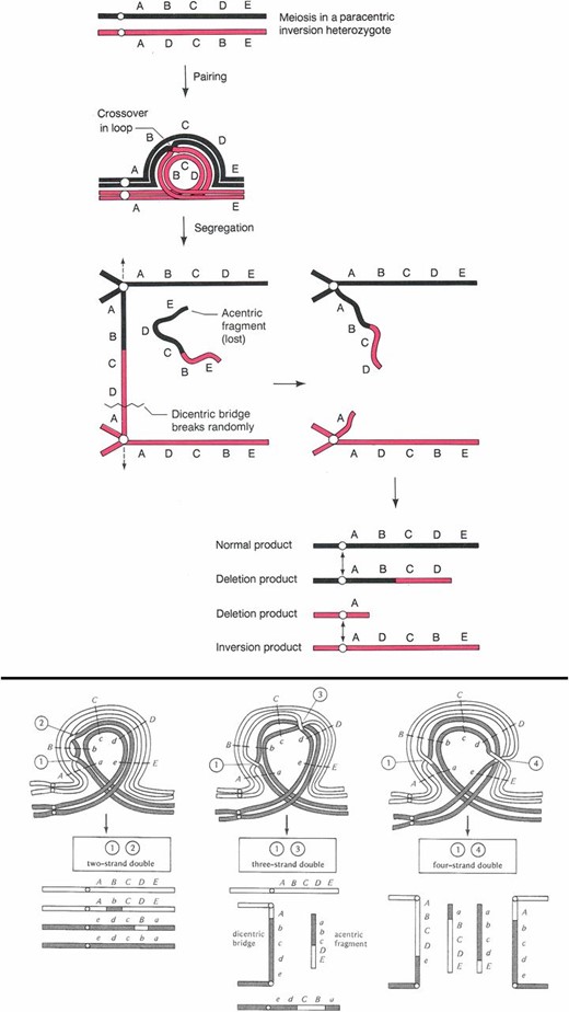
Diagrammatic representation of the paring configuration and consequences of crossing over in a female heterozygous for a paracentric inversion. At the top the pairing configuration is shown as a loop. A single crossover within the loop results in the formation of a dicentric bridge and an acentric fragment at the first meiotic division. The bridge can break at random positions and the acentric fragment is lost. The result of this single exchange is the production of two euploid progeny, one inverted and the other normal. The other two meiotic products are grossly aneuploid and are unlikely to support normal development if used. Below the single exchange diagram are shown the results of double exchanges within the paired inversion loop. If a double exchange takes place between the same pair of chromatids (two-strand double), the interval between the two crossovers will be exchanged between the inverted and normal sequence homologs and all euploid products will be formed. If the double exchange occurs between an odd number of chromatids (three-strand double) or all four (four-strand double), like single crossover bridges and fragments are formed, grossly aneuploid meiotic products will be formed. After Griffiths et al. (2000) and Strickberger (1976). The letters aligned with the chromosomes indicate the positions of genes.
Heterozygosity for a pericentric inversion is also associated with the recovery of aneuploid gametes but by a different mechanism. Single-exchange events within the inversion loop do not form bridges but rather produce chromatids that are grossly duplicated and deleted for large portions of the chromosome arms (Figure 10). Again, if these gametes are used in fertilization, the resultant progeny will also be grossly aneuploid and lethal. Similar to the case of the paracentric inversions, two-strand double-exchange events can be recovered and can be used to transfer genes in and out of inversion-bearing chromosomes.
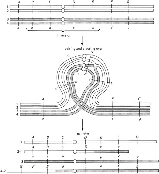
Diagrammatic representation of the consequences of crossing over in a female heterozygous for a pericentric inversion. As for the paracentric inversion, paring occurs in a loop but in this case the centromere is within the inverted region. Exchange events in the paired inverted region produce gametes that are grossly aneuploid for large portions of whole chromosome arms. These aneuploid gametes are incapable of producing viable progeny if used in fertilization. Unlike the paracentric inversions there are no anaphase bridges and acentric fragments produced. After Strickberger (1976). The letters and hash marks along the chromosome arms indicate the position of genes.
The next class of chromosomal aberrations is translocations. In a sense, the Y-linked duplications mentioned above are a kind of translocation called nonreciprocal. Reciprocal translocations are those in which two chromosome arms or portions of arms are exchanged (Figure 11). An animal homozygous for a viable reciprocal translocation will show a difference in linkage groups, moving the genes in the translocated arms into different linkage relationships than those seen in a normal wild-type genotype. Heterozygosity for a translocation has no effect on somatic cell division but dramatically disrupts meiosis in both males and females. Pairing in meiosis I is in the form of a cross (Figure 11). From this pairing configuration, there are three possible segregation patterns. The first, Alternate disjunction, results in the segregation of the translocated elements to one pole and the normal chromosome complement to the other, thereby creating euploid balanced gametes. The second and third patterns are called Adjacent 1 and 2. Both of these disjunction and segregation patterns result in the production of gametes containing a mixture of translocation and nontranslocation chromosomes, and are thus unbalanced and aneuploid with massive deletions and duplications of genetic material. The frequency of Alternate disjunction is ∼50% with the two forms of Adjacent disjunction comprising the remainder. Since only the Alternate pattern produces euploid gametes, translocation heterozygotes (male and female) have their fertility lowered by 50%.
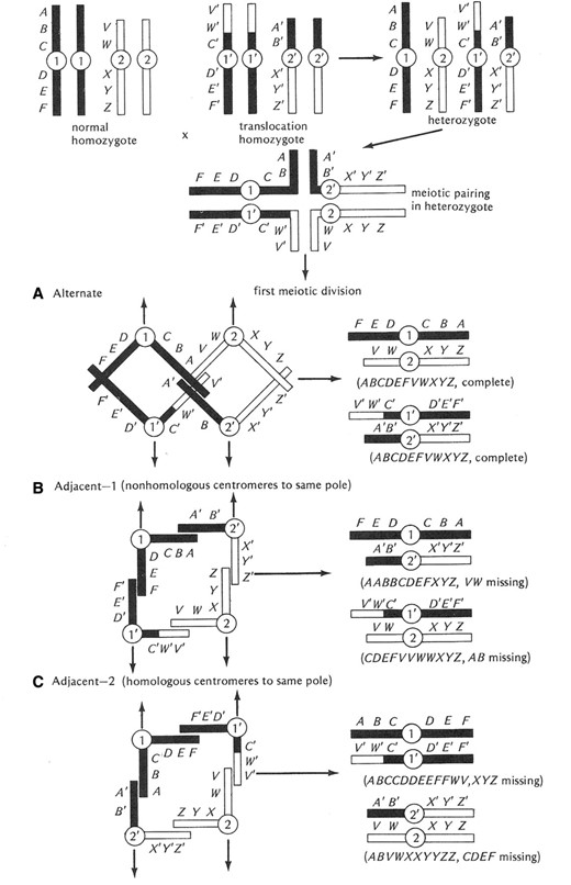
Diagrammatic representation of the consequences of heterozygosity for a simple reciprocal translocation. Both male and female heterozygotes for a translocation pair in the form of a cross (shown at the top of the figure). The major consequences of translocation heterozygosity are associated with the three potential patterns of segregation of the centromeres of the translocation and normal homologs. The first type, called Alternate (A) disjunction, results in the segregation of the two normal homologs and the two translocation elements to the opposite poles in the first meiotic division. The resultant gametes are euploid or balanced and will produce viable progeny. The other patterns of segregation, Adjacent 1 (B) and Adjacent 2 (C), result in one of the translocation elements and one of the normal chromosomes migrating to the same pole. Both Adjacent patterns result in the production of grossly aneuploid gametes that are incapable of producing viable progeny. The Alternate and Adjacent patterns occur in a 1:1 ratio and result in heterozygotes having 50% fertility relative to either homozygous condition. After Strickberger (1976). The letters along the chromosomes indicate the position of genes.
The final category of structural change is the compound chromosome. In actual fact, these specialized chromosomes can be viewed as translocations. Perhaps the most widely known are the compound X chromosomes. In this case, since the two homologous XL arms are joined, this configuration can only be found in females. The X chromosomes may be joined together in six ways and the configurations are named based on the position of the centromere and the relative gene order in the two arms. When the centromere is located centrally the compound is referred to as metacentric, and when the centromere is located at the end it is called an acrocentric. Additionally, the order of the two X chromosome arms can be tandem or reversed. Thus, there are the four basic types with a free arm or arms and two ends: reversed metacentric, tandem metacentric, reversed acrocentric, and tandem acrocentric (see Table 3). In addition to these there are two compound rings, Tandem Ring C(1)TR and Reversed Ring C(1)RR, which will not be considered further here (Novitski 1954).
The four basic types of X chromosome attachments
| Reversed metacentric | C(1)RM | Telomere———–•———–Telomere |
| Tandem metacentric | C(1)TM | Telomere———–•Telomere———– |
| Reversed acrocentric | C(1)RA | Telomere———————-Telomere• |
| Tandem acrocentric | C(1)TA | Telomere———–Telomere———–• |
| Reversed metacentric | C(1)RM | Telomere———–•———–Telomere |
| Tandem metacentric | C(1)TM | Telomere———–•Telomere———– |
| Reversed acrocentric | C(1)RA | Telomere———————-Telomere• |
| Tandem acrocentric | C(1)TA | Telomere———–Telomere———–• |
| Reversed metacentric | C(1)RM | Telomere———–•———–Telomere |
| Tandem metacentric | C(1)TM | Telomere———–•Telomere———– |
| Reversed acrocentric | C(1)RA | Telomere———————-Telomere• |
| Tandem acrocentric | C(1)TA | Telomere———–Telomere———–• |
| Reversed metacentric | C(1)RM | Telomere———–•———–Telomere |
| Tandem metacentric | C(1)TM | Telomere———–•Telomere———– |
| Reversed acrocentric | C(1)RA | Telomere———————-Telomere• |
| Tandem acrocentric | C(1)TA | Telomere———–Telomere———–• |
The reversed types can pair by a forming a hairpin configuration of the two arms, while the tandem types pair in a loop or ring-like alignment. Both of the tandem configurations are unstable and are resolved into a normal single X by recombination. The reversed configuration is more stable and thus more useful. The first compound X was discovered by L. V. Morgan, T. H. Morgan’s wife, in 1938 (Morgan 1938) and was a C(1)RM. The RM type compound has been very useful in the analysis of recombination in that two of the four chromatids involved in an exchange tetrad can be recovered in the same oocyte nucleus and half tetrad analysis can be performed. Additionally, the pattern of chromosomal inheritance allowing the recovery of patroclinous males and matroclinous females has been useful in simplifying genetic screens on the X (Figure 12).
![(A) Diagram of the karyotypes of normal and attached X females and the pattern of inheritance of the attachment. In an attached X female both normally acrocentric X arms are associated with a single centromere. Shown at the top is the normal karyotype, below that is an example of a Compound Reverse Metacentric [C(1)RM]. The Punnett Square shows the gametes produced by a C(1)RM/Y female on the left and a normal X/Y male above the square. Unlike the normal “crisscross” pattern of the sex chromosome pattern of inheritance, the daughters inherit their X chromosomes from their mother (matroclinous inheritance) and the sons inherit their X from their father (patroclinous inheritance). Only the Y chromosomes are exchanged to the opposite sex. Also note that the XXX and YY progeny die. Thus, only 50% of the zygotes from an attached X cross survive. (B) Diagram of karyotypes of compound autosome and the gamete types produced by compound-bearing animals. The normally metacentric autosomes can be fused or translocated at the centromere such that the left and right arms are now attached. At the top left a Compound 2L;2R female [C(2L);C(2R)], and to the right a Compound 3L;3R male [C(3L);C(3R)] are shown. Below, the Punnett Square presents the gametes produced in females and males carrying C(2L);C(2R). Females segregate the two compound arms 100% of the time and thus form two types of ova: C(2L) and C(2R). Males on the other hand form all four potential types of sperm in equal frequency. The only viable progeny are formed when reciprocal meiotic segregation products join: C(2L) + C(2R). All other combinations are grossly aneuploidy and lethal. Note that any cross of a compound-bearing male or female to a normal animal will be essentially sterile. The only exception is if a compound-bearing male C(2L);C(2R) or O;O sperm fertilize a reciprocal nullo-2 or diplo-2 ovum produced by nondisjunction in the mated female.](https://oup.silverchair-cdn.com/oup/backfile/Content_public/Journal/genetics/206/2/10.1534_genetics.117.199950/5/m_665fig12.jpeg?Expires=1716395907&Signature=L2h6V4I3o2Y7WYdwaRMbGIoBYWhSIzzcz-JY6FBkg-uNrJfxUmxReNiCiSUXfBxxfNBrXLFjp8KTzwnDpXBjiin7NnFpQP3kLKSbNd7h2LNw-mVYbWeolXm43Iw0IDdDQW0ac-EMMpACkT8WuJ6GD3bTs7OGRuxBmyDbV4rdnqhvdGEFek8FQyQBSK9VedoK0yBOFXf1fT6s69VhzxuH~adEsl7V5dnvxZYXpxOLYlF29D~O~Dy1-9lrDqYEpk0oDOlsNNhFDDhTNZRDFWK7sE9nUIKYXlgT0674rpFz4w9z94~xe7CYdCFBV5FI5J8YnKi74YuERH73KPD857E0fQ__&Key-Pair-Id=APKAIE5G5CRDK6RD3PGA)
(A) Diagram of the karyotypes of normal and attached X females and the pattern of inheritance of the attachment. In an attached X female both normally acrocentric X arms are associated with a single centromere. Shown at the top is the normal karyotype, below that is an example of a Compound Reverse Metacentric [C(1)RM]. The Punnett Square shows the gametes produced by a C(1)RM/Y female on the left and a normal X/Y male above the square. Unlike the normal “crisscross” pattern of the sex chromosome pattern of inheritance, the daughters inherit their X chromosomes from their mother (matroclinous inheritance) and the sons inherit their X from their father (patroclinous inheritance). Only the Y chromosomes are exchanged to the opposite sex. Also note that the XXX and YY progeny die. Thus, only 50% of the zygotes from an attached X cross survive. (B) Diagram of karyotypes of compound autosome and the gamete types produced by compound-bearing animals. The normally metacentric autosomes can be fused or translocated at the centromere such that the left and right arms are now attached. At the top left a Compound 2L;2R female [C(2L);C(2R)], and to the right a Compound 3L;3R male [C(3L);C(3R)] are shown. Below, the Punnett Square presents the gametes produced in females and males carrying C(2L);C(2R). Females segregate the two compound arms 100% of the time and thus form two types of ova: C(2L) and C(2R). Males on the other hand form all four potential types of sperm in equal frequency. The only viable progeny are formed when reciprocal meiotic segregation products join: C(2L) + C(2R). All other combinations are grossly aneuploidy and lethal. Note that any cross of a compound-bearing male or female to a normal animal will be essentially sterile. The only exception is if a compound-bearing male C(2L);C(2R) or O;O sperm fertilize a reciprocal nullo-2 or diplo-2 ovum produced by nondisjunction in the mated female.
It is also possible to form compound chromosomes involving the autosomal complement. In this case, the normally metacentric second and third chromosomes are reconfigured so that the homologous Left and Right arms are attached to the same centromere (Figure 12). The nomenclature used is C(2L);C(2R) and C(3L);C(3R) (Holm and Chovnick 1975; Holm 1976). This configuration has interesting consequences in meiosis. Males carrying a pair of compounds for chromosome 2 produce all four potential gametes (Figure 12). Females on the other hand produce only two that carry either the C(2L) or C(2R). When these males and females are crossed, only 25% of the resulting progeny are euploid and thus viable. It is also the case that if either sex is crossed to a normal noncompound animal, the cross is essentially sterile. The only exception would be if a compound male were crossed and one of his double-compound or double-nullo sperm were to fertilize an egg that was nullo or disomic as a result of nondisjunction in the female parent. While this is possible it is exceedingly rare. Nonetheless, such a cross can be used for the very efficient recovery of nondisjunction events in females carrying meiotic mutations or different chromosomal configurations. Like the C(1)RM, the autosomal compounds can be used effectively in the analysis of recombination by the recovery of half tetrads rather than single chromatids. However, they do have a distinct advantage over the compound X situation. Markers for the analysis of exchange events can be inserted into a compound pair, which in such an analysis must begin in a heterozygous configuration. Unfortunately, exchange events that take place in the C(1)RM proximal to the gene or genes being analyzed will result in homozygosity for those markers making the genotype useless in the analysis. The further the markers are from the centromere the more likely they will become homozygous. This problem is overcome in the case of the autosomal compounds because the heterozygous configuration can be maintained by keeping that state in males where recombination does not take place. The construction of compound autosomes has been taken to its logical extreme by the recovery of C(2)EN, C(3)EN, and C(2;3)EN configurations (Novitski et al. 1981). C(2)EN and C(3)EN attach the entirety of chromosomes 2 and 3, respectively, to a single centromere, while C(2;3)EN attaches the entire major autosomal compliment to a single centromere. The fertility of these compounds is low and they thus are difficult to culture and work with. Nonetheless, they are testament to the dramatic extent to which the fly genome can be manipulated and reconfigured.
Balancers
In addition to the polytene chromosomes, Drosophila provides another extremely valuable tool to the geneticist: these are the balancer chromosomes. These chromosomes serve two important purposes. The first is allowing the maintenance of lethal and sterile mutations in stock without selection. The second is that they can be used in screens for mutations by maintaining the linear integrity of a mutagenized homolog. How do they do this? An answer comes from understanding their constituent parts. Balancers contain one or more inverted sequences relative to a normal chromosome to prevent the recovery of exchange events, thus isolating and maintaining the sequences in the balancer and the balanced chromosome. Note that they do not prevent crossing over but inhibit the recovery of exchange chromatids. The above discussion of the meiotic effects of inversions demonstrates how this is accomplished. Exchange events within the paired loop of a paracentric inversion creates anaphase bridges and, due to the polarized nature of female meiosis, the bridge constrains the exchange chromatids into the central pair of polar body nuclei (Sturtevant and Beadle 1936; Figure 13). Pericentric inversions also prevent the recovery of exchange chromatids by virtue of the production of grossly aneuploid gametes that produce lethal progeny. The original balancer chromosomes were associated with single inversions, e.g., In(1)dl-49 and ClB (Table 4). While these simple balancers were reasonably efficient they were not perfect. Double crossovers within the inversion loop could result in exchange of material between the balancer and its homolog, and exchange events outside the inversion were also possible. This limitation was overcome by combining inversions, i.e., creating inversions within inversions or creating overlapping inversions. This was done in two ways: (1) genetically by the recovery of rare double exchange events between two inversions, e.g., inserting a smaller inversion into the sequence of a larger aberration, or (2) mutationally by the irradiation of simple inversions to recover superimposed additional inversions. Both methods worked and produced the array of balancers listed in Table 4. This list is not all inclusive and additional balancers can be found at the BDSC (http://flystocks.bio.indiana.edu/Browse/balancers/balancer_main.htm).
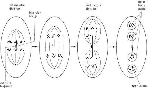
The mechanism by which paracentric inversions prevent the recovery of crossover chromatids in females. At fertilization, meiosis is completed in the oocyte. The axis of the meiotic spindle forms perpendicular to the surface of the egg. If an exchange has taken place within the inverted sequence, the bridge formed constrains the involved chromatids to the center of the first meiotic anaphase. At the second division, the exchange chromatids are confined to the central nuclei while the nonexchange chromatids are segregated into the nuclei at the two ends of the polarized meiotic spindle. The fragment associated with the bridge is lost in the middle of the polar spindle. The inner-most haploid nucleus, the one furthest from the egg surface, is always the one that is used as the oocyte nucleus and will participate in syngamy. Thus, heterozygosity for a paracentric inversion does not prevent crossing over but rather prevents the recovery of crossover chromatids by constraining them to the central two nuclear products of the polarized meiotic spindle. After Strickberger (1976).
Listing of some of the most commonly-used balancer chromosomes
| Balancer Symbols | Markers | Cytological Order |
|---|---|---|
| In(1)dl-49 | In(1)dl-49, y Hw m2 g4 | 1A - 4D7 | 11F2 - 4E1 | 11F4 - 20F• |
| Basc | In(1)scS1Lsc8R+S, sc8 scS1 wa B1 | 1A - 1B3 | 20F - 11A1 | 6F - 10F10 | 6F - 1B3 | 20F• |
| Binsinscy | In(1)scS1Lsc8R+dl-49, yc4 sc8 scS1 w1 snX2 B1 | 1A - 1B3 | 20F - 11F4 | 4E1 - 11F2 | 4D7 - 1B3 | 20F• |
| ClB | In(1)Cl, sc1 l(1)C1 t2 v1 sl1 B1 | 1A - 4A5 | 17A6 - 4B1 | 17A6 - 20F• |
| FM0 | In(1)sc8+dl-49, y31d sc8 w1 vOf m2 f1 B1 | 1A - 1B2 | 20F - 11F4 | 4E1 - 11F2 | 4D7 - 1B2 | 20F - 20F• |
| FM3 | In(1)FM3, y31d sc8 dm1 B1 | 1A - 1B2 | 20F | 16B - 19F | 3F - 4D7 | 11F2 - 4E1 | 11F4 - 16A | 3E - 1B3 | 20F• |
| FM4 | In(1)FM4, y31d sc8 dm1 B1 | 1A - 1B2 | 20F - 11F4 | (4E - 4E) | 3C - 4D7 | 11F2 - 4F | 3C - 1B3 | 20F• |
| FM6 | In(1)FM6, y31d sc8 dm1 B1 | 1A - 1B2 | (20B - 20B) | 15E - 21A | 15D - 11F4 | (4E - 4E) | 3C - 4D7 | 11F2 - 4F | 3C - 1B3 | 20D1 - 20F• |
| FM7a | In(1)FM7, y31d sc8 wa vOf B1 | 1A - 1B2 | 20F - 21A | 15D - 21A | 15D - 11F4 | 4E1 - 11F2 | 4D7 - 1B3 | 20F• |
| FM7b | In(1)FM7, y31d sc8 wa lzs B1 | 1A - 1B2 | 20F - 21A | 15D - 21A | 15D - 11F4 | 4E1 - 11F2 | 4D7 - 1B3 | 20F• |
| FM7c | In(1)FM7, y31d sc8 wa snX2 vOf g4 B1 | 1A - 1B2 | 20F - 21A | 15D - 21A | 15D - 11F4 | 4E1 - 11F2 | 4D7 - 1B3 | 20F• |
| FM7d | In(1)FM7, y31d sc8 B1 | 1A - 1B2 | 20F - 21A | 15D - 21A | 15D - 11F4 | 4E1 - 11F2 | 4D7 - 1B3 | 20F• |
| FM7h | In(1)FM7, y31d sc8 w1 oc1 ptg1 B1 | 1A - 1B2 | 20F - 21A | 15D - 21A | 15D - 11F4 | 4E1 - 11F2 | 4D7 - 1B3 | 20F• |
| FM7i | In(1)FM7, y93j sc8 w1 oc1 ptg1 B1 | 1A - 1B2 | 20F - 21A | 15D - 21A | 15D - 11F4 | 4E1 - 11F2 | 4D7 - 1B3 | 20F• |
| FM7j | In(1)FM7, y93j sc8 w1 | 1A - 1B2 | 20F - 21A | 15D - 21A | 15D - 11F4 | 4E1 - 11F2 | 4D7 - 1B3 | 20F• |
| FM7k | In(1)FM7, y31d sc8 snX2 B1 | 1A - 1B2 | 20F - 21A | 15D - 21A | 15D - 11F4 | 4E1 - 11F2 | 4D7 - 1B3 | 20F• |
| CyO | In(2LR)O, Cy1 dplvI pr1 cn2 | 21A - 22D1 | 33F5 - 30F | 50D1 - 58A4 | 42A2 • 34A1 | 22D2 - 30E | 50C10 - 42A3 | 58B1 - 60F |
| SM1 | In(2LR)SM1, al2 Cy1 cn2 sp2 | 21A - 22A3 | 60B - 58B1 | 42A3 - 58A4 | 42A2 • 34A1 | 22D2 - 33F5 | 22D1 - 22B1 | 60C - 60F |
| SM5 | In(2LR)SM5, al2 ds55 Cy1 ltv cn2 sp2 | 21A - 21D2 | 36C - 40F | 29C - 22D2 | 34A1 - 36C | 21D3 - 22A3 | 60B - 58B1 | 42A3 - 42D | 42D - 42A3 | 58B1 - 58F | 53C - 42D | 53C - 58A4 | 42A2 • 40F | 29E - 33F5 | 22D1 - 22B1 | 60C - 60F |
| SM6a | In(2LR)SM6, al1 Cy1 dplvI cn2P sp2 | 21A - 22A3 | 60B - 58B1 | 42A3 - 50C10 | 30E - 22D | 34A1 • 42A2 | 58A4 - 50D1 | 30F - 33F5 | 22D1 - 22B1 | 60C - 60F |
| SM6b | In(2LR)SM6, Roi1, al1 Cy1 dplvI cn2P sp2 | 21A - 22A3 | 60B - 58B1 | 42A3 - 50C10 | 30E - 22D | 34A1 • 42A2 | 58A4 - 50D1 | 30F - 33F5 | 22D1 - 22B1 | 60C - 60F |
| CxD | In(3LR)CxD, D1 | 61A - 69D3 | 70C13 - 69E1 | 70D1 - 71F | 85C - 84A | 80 • 84A | 93F - 85C | 71F - 80 | 93F - 100F |
| LVM | In(3L)P, In(3R)P, l(3)LVML1pe1 l(3)LVMR1, PoLVM | 61A - 63B8 | 72E1 - 63B9 | 72E2 • 89C2 | 96A18 - 89C3 | 96A19 - 100F |
| MKRS | Tp(3;3)MRS, M(3)76A1 kar1 ry2 Sb1 | 61A - 71B2 | 92E - 93C | 87F1 - 92E | 71C2 • 87E8 | 93C - 100F |
| TM1 | In(3LR)TM1, Me1 kniri−1 Sbsbd-l | 61A - 63C | 72E1 - 69E | 91C - 97D | 89B • 72E2 | 63C - 69E | 91C - 89B | 97D - 100F |
| TM2 | In(3LR)Ubx130, emc2 Ubx130 es | 61A - 61A | 96B - 93B | 89D • 74 | 61C - 74 | 89E - 93B | 96A - 100F |
| TM3 | In(3LR)TM3, kniri−1 pp sep1 l(3)89Aa1 Ubxbx−34e e1 | 61A - 65E | 85E • 79E | 100C - 100F2 | 92D1 - 85E | 65E - 71C | 94D - 93A | 76C - 71C | 94F - 100C | 79E - 76C | 93A - 92E1 | 100F3 - 100F |
| TM6 | In(3LR)TM6, HnP ssP88 bx34e UbxP15 e1 | 61A - 61A | 89C2 • 75C | 94A - 100F2 | 92D1 - 89C4 | 61A2 - 63B8 | 72E1 - 63B11 | 72E2 - 75C | 94A - 92E1 | 100F3 - 100F |
| TM6B | In(3LR)TM6B, AntpHu e1 | 61A - 61A1 | 87B2 - 86C8 | 84F2 - 86C7 | 84B2 - 84F2 | 84B2 • 75C | 94A - 100F2 | 92D1 - 87B4 | 61A2 - 63B8 | 72E1 - 63B11 | 72E2 - 75C | 94A - 92E1 | 100F3 - 100F |
| TM6B, Tb | In(3LR)TM6B, AntpHu e1 Tb1 | 61A - 61A1 | 87B2 - 86C8 | 84F2 - 86C7 | 84B2 - 84F2 | 84B2 • 75C | 94A - 100F2 | 92D1 - 87B4 | 61A2 - 63B8 | 72E1 - 63B11 | 72E2 - 75C | 94A - 92E1 | 100F3 - 100F |
| TM6C | In(3LR)TM6C, e1 | 61A - 61A1 | 87B2 • 75C | 94A - 100F2 | 92D1 - 87B4 | 61A2 - 63B8 | 72E1 - 63B9 | 72E2 - 75C | 94A - 92D9 | 100F3 - 100F |
| TM8 | In(3LR)TM8, l(3)DTS41 th1 st1 Sb1 e1 | 61A - 62D2 | 80C - 73F | 87D2 • 80C | 62D7 - 73F | 87D3 - 92D1 | 100F2 - 92E1 | 100F3 - 100F |
| TM9 | In(3LR)TM9, l(3)DTS41 th1 st1 Sb1 e1 | 61A - 62D2 | 85A - 87A | 76F - 80C | 85A • 80C | 62D7 - 76F | 87A - 92D1 | 100F2 - 92E1 | 100F3 - 100F |
The first column lists the abbreviation for the balancer. FM, First Multiple; SM, Second Multiple; TM, Third Multiple; the others are named for their genic content. The second column shows the genotype, name of the inversion or inversion complexes, and markers in the balancer. The third column shows the new order of segments of the chromosome using Bridges’ coordinate system. The pipes indicate the position of a breakpoint and the black dot the position of the centromere. A more complete listing of balancers can be found at: http://flystocks.bio.indiana.edu/Browse/balancers/balancer_main.htm.
| Balancer Symbols | Markers | Cytological Order |
|---|---|---|
| In(1)dl-49 | In(1)dl-49, y Hw m2 g4 | 1A - 4D7 | 11F2 - 4E1 | 11F4 - 20F• |
| Basc | In(1)scS1Lsc8R+S, sc8 scS1 wa B1 | 1A - 1B3 | 20F - 11A1 | 6F - 10F10 | 6F - 1B3 | 20F• |
| Binsinscy | In(1)scS1Lsc8R+dl-49, yc4 sc8 scS1 w1 snX2 B1 | 1A - 1B3 | 20F - 11F4 | 4E1 - 11F2 | 4D7 - 1B3 | 20F• |
| ClB | In(1)Cl, sc1 l(1)C1 t2 v1 sl1 B1 | 1A - 4A5 | 17A6 - 4B1 | 17A6 - 20F• |
| FM0 | In(1)sc8+dl-49, y31d sc8 w1 vOf m2 f1 B1 | 1A - 1B2 | 20F - 11F4 | 4E1 - 11F2 | 4D7 - 1B2 | 20F - 20F• |
| FM3 | In(1)FM3, y31d sc8 dm1 B1 | 1A - 1B2 | 20F | 16B - 19F | 3F - 4D7 | 11F2 - 4E1 | 11F4 - 16A | 3E - 1B3 | 20F• |
| FM4 | In(1)FM4, y31d sc8 dm1 B1 | 1A - 1B2 | 20F - 11F4 | (4E - 4E) | 3C - 4D7 | 11F2 - 4F | 3C - 1B3 | 20F• |
| FM6 | In(1)FM6, y31d sc8 dm1 B1 | 1A - 1B2 | (20B - 20B) | 15E - 21A | 15D - 11F4 | (4E - 4E) | 3C - 4D7 | 11F2 - 4F | 3C - 1B3 | 20D1 - 20F• |
| FM7a | In(1)FM7, y31d sc8 wa vOf B1 | 1A - 1B2 | 20F - 21A | 15D - 21A | 15D - 11F4 | 4E1 - 11F2 | 4D7 - 1B3 | 20F• |
| FM7b | In(1)FM7, y31d sc8 wa lzs B1 | 1A - 1B2 | 20F - 21A | 15D - 21A | 15D - 11F4 | 4E1 - 11F2 | 4D7 - 1B3 | 20F• |
| FM7c | In(1)FM7, y31d sc8 wa snX2 vOf g4 B1 | 1A - 1B2 | 20F - 21A | 15D - 21A | 15D - 11F4 | 4E1 - 11F2 | 4D7 - 1B3 | 20F• |
| FM7d | In(1)FM7, y31d sc8 B1 | 1A - 1B2 | 20F - 21A | 15D - 21A | 15D - 11F4 | 4E1 - 11F2 | 4D7 - 1B3 | 20F• |
| FM7h | In(1)FM7, y31d sc8 w1 oc1 ptg1 B1 | 1A - 1B2 | 20F - 21A | 15D - 21A | 15D - 11F4 | 4E1 - 11F2 | 4D7 - 1B3 | 20F• |
| FM7i | In(1)FM7, y93j sc8 w1 oc1 ptg1 B1 | 1A - 1B2 | 20F - 21A | 15D - 21A | 15D - 11F4 | 4E1 - 11F2 | 4D7 - 1B3 | 20F• |
| FM7j | In(1)FM7, y93j sc8 w1 | 1A - 1B2 | 20F - 21A | 15D - 21A | 15D - 11F4 | 4E1 - 11F2 | 4D7 - 1B3 | 20F• |
| FM7k | In(1)FM7, y31d sc8 snX2 B1 | 1A - 1B2 | 20F - 21A | 15D - 21A | 15D - 11F4 | 4E1 - 11F2 | 4D7 - 1B3 | 20F• |
| CyO | In(2LR)O, Cy1 dplvI pr1 cn2 | 21A - 22D1 | 33F5 - 30F | 50D1 - 58A4 | 42A2 • 34A1 | 22D2 - 30E | 50C10 - 42A3 | 58B1 - 60F |
| SM1 | In(2LR)SM1, al2 Cy1 cn2 sp2 | 21A - 22A3 | 60B - 58B1 | 42A3 - 58A4 | 42A2 • 34A1 | 22D2 - 33F5 | 22D1 - 22B1 | 60C - 60F |
| SM5 | In(2LR)SM5, al2 ds55 Cy1 ltv cn2 sp2 | 21A - 21D2 | 36C - 40F | 29C - 22D2 | 34A1 - 36C | 21D3 - 22A3 | 60B - 58B1 | 42A3 - 42D | 42D - 42A3 | 58B1 - 58F | 53C - 42D | 53C - 58A4 | 42A2 • 40F | 29E - 33F5 | 22D1 - 22B1 | 60C - 60F |
| SM6a | In(2LR)SM6, al1 Cy1 dplvI cn2P sp2 | 21A - 22A3 | 60B - 58B1 | 42A3 - 50C10 | 30E - 22D | 34A1 • 42A2 | 58A4 - 50D1 | 30F - 33F5 | 22D1 - 22B1 | 60C - 60F |
| SM6b | In(2LR)SM6, Roi1, al1 Cy1 dplvI cn2P sp2 | 21A - 22A3 | 60B - 58B1 | 42A3 - 50C10 | 30E - 22D | 34A1 • 42A2 | 58A4 - 50D1 | 30F - 33F5 | 22D1 - 22B1 | 60C - 60F |
| CxD | In(3LR)CxD, D1 | 61A - 69D3 | 70C13 - 69E1 | 70D1 - 71F | 85C - 84A | 80 • 84A | 93F - 85C | 71F - 80 | 93F - 100F |
| LVM | In(3L)P, In(3R)P, l(3)LVML1pe1 l(3)LVMR1, PoLVM | 61A - 63B8 | 72E1 - 63B9 | 72E2 • 89C2 | 96A18 - 89C3 | 96A19 - 100F |
| MKRS | Tp(3;3)MRS, M(3)76A1 kar1 ry2 Sb1 | 61A - 71B2 | 92E - 93C | 87F1 - 92E | 71C2 • 87E8 | 93C - 100F |
| TM1 | In(3LR)TM1, Me1 kniri−1 Sbsbd-l | 61A - 63C | 72E1 - 69E | 91C - 97D | 89B • 72E2 | 63C - 69E | 91C - 89B | 97D - 100F |
| TM2 | In(3LR)Ubx130, emc2 Ubx130 es | 61A - 61A | 96B - 93B | 89D • 74 | 61C - 74 | 89E - 93B | 96A - 100F |
| TM3 | In(3LR)TM3, kniri−1 pp sep1 l(3)89Aa1 Ubxbx−34e e1 | 61A - 65E | 85E • 79E | 100C - 100F2 | 92D1 - 85E | 65E - 71C | 94D - 93A | 76C - 71C | 94F - 100C | 79E - 76C | 93A - 92E1 | 100F3 - 100F |
| TM6 | In(3LR)TM6, HnP ssP88 bx34e UbxP15 e1 | 61A - 61A | 89C2 • 75C | 94A - 100F2 | 92D1 - 89C4 | 61A2 - 63B8 | 72E1 - 63B11 | 72E2 - 75C | 94A - 92E1 | 100F3 - 100F |
| TM6B | In(3LR)TM6B, AntpHu e1 | 61A - 61A1 | 87B2 - 86C8 | 84F2 - 86C7 | 84B2 - 84F2 | 84B2 • 75C | 94A - 100F2 | 92D1 - 87B4 | 61A2 - 63B8 | 72E1 - 63B11 | 72E2 - 75C | 94A - 92E1 | 100F3 - 100F |
| TM6B, Tb | In(3LR)TM6B, AntpHu e1 Tb1 | 61A - 61A1 | 87B2 - 86C8 | 84F2 - 86C7 | 84B2 - 84F2 | 84B2 • 75C | 94A - 100F2 | 92D1 - 87B4 | 61A2 - 63B8 | 72E1 - 63B11 | 72E2 - 75C | 94A - 92E1 | 100F3 - 100F |
| TM6C | In(3LR)TM6C, e1 | 61A - 61A1 | 87B2 • 75C | 94A - 100F2 | 92D1 - 87B4 | 61A2 - 63B8 | 72E1 - 63B9 | 72E2 - 75C | 94A - 92D9 | 100F3 - 100F |
| TM8 | In(3LR)TM8, l(3)DTS41 th1 st1 Sb1 e1 | 61A - 62D2 | 80C - 73F | 87D2 • 80C | 62D7 - 73F | 87D3 - 92D1 | 100F2 - 92E1 | 100F3 - 100F |
| TM9 | In(3LR)TM9, l(3)DTS41 th1 st1 Sb1 e1 | 61A - 62D2 | 85A - 87A | 76F - 80C | 85A • 80C | 62D7 - 76F | 87A - 92D1 | 100F2 - 92E1 | 100F3 - 100F |
The first column lists the abbreviation for the balancer. FM, First Multiple; SM, Second Multiple; TM, Third Multiple; the others are named for their genic content. The second column shows the genotype, name of the inversion or inversion complexes, and markers in the balancer. The third column shows the new order of segments of the chromosome using Bridges’ coordinate system. The pipes indicate the position of a breakpoint and the black dot the position of the centromere. A more complete listing of balancers can be found at: http://flystocks.bio.indiana.edu/Browse/balancers/balancer_main.htm.
The second feature of the balancers relates to their genic content. To effectively balance lethal and sterile mutations they should contain a recessive lethal mutation not related to the lesion being balanced. It is also useful for the balancer to carry a dominant visible mutation so that it can be easily followed in crossing schemes and animals carrying the balancer can be easily distinguished. Many balancers also carry sets of recessive visible mutations that can be useful in designing screens and discerning complex genotypes. The advent of transgenesis has added a new set of markers to the balancer repertoire. Transgenically-inserted fragments expressing LacZ, GFP, or other fluorophores in a variety of spatiotemporal patterns have been inserted into different preexisting balancers, adding new and useful dominant markers that can be used to distinguish balancer from nonbalancer animals at different developmental stages. It should be noted that one does not have to use balancers for the fourth chromosome. This element does not normally crossover, i.e., it is achiasmatic in females. Thus, to maintain a balanced stock for a lethal or sterile mutation on chromosome 4 it is sufficient to use a normal sequenced four marked with a dominant visible mutation and a recessive lethal.
As useful as the multiply-inverted balancers are, they still do not offer absolute protection against the recovery of exchange products and the breakdown of a balanced lethal stock. When choosing a balancer to maintain an important lethal or sterile, it is important to consider the location of the gene to be balanced relative to the sequence of the balancer. It is always best to pick a balancer that has a breakpoint close to the gene to be balanced. A gene in the center of a large inversion can be exchanged by a double crossover. Additionally, genes near the telomere are not always well-maintained, especially if the balancer used does not have a break near the end of the chromosome. A case in point is TM3 (Table 4). The 3L telomere at 61A has, as its closest break 65E, five numbered units removed leaving 20% of 3L uninterrupted. The original TM3 had a small tip of the X chromosome appended at 61A containing the y+ locus, which could be used as a marker to follow the balancer in a y− background. Most TM3 lines currently held in stock have lost this marker, showing that TM3 should not be used to maintain lesions known to reside in the 61–64 interval.
Genetic Screens
In the early days of Drosophila genetics, new mutations were found as serendipitous spontaneous occurrences. Methods developed in attempts to take the randomness out of mutation discovery were labor intensive and involved complicated sets of progeny testing crosses. The fact that spontaneous mutation rates were low made this all the more difficult: “Lots of chaff little wheat.” This all changed with Muller’s discovery that X-rays were mutagenic, elevating the mutation rate by orders of magnitude (Muller 1928). Coupled with this discovery was the building-set of tools in the hands of the Morgan lab. One of these was the discovery of an X chromosome that appeared to suppress crossing over on the X in a dominant fashion called “C.” Also, the dominant eye shape mutation Bar was recovered. In addition to suppressing crossing over, the C chromosome was found to possess a recessive lethal preventing its recovery in males. The combination of the C chromosome with Bar was the first instance of a balancer and Muller took advantage of it in designing the first directed screen for sex-linked lethals. As shown in Figure 14, adult males are irradiated and crossed to ClB/+++ females. In the F1 progeny, ClB/+*+*+* females are singly mated to normal males. Single females are used in this cross because each female is the product of a single irradiated sperm. In the next F2 generation the heterozygous ClB females survive while the ClB/Y male siblings die. If a new lethal mutation is induced in the sperm of the P1 male parent, then there will be no male progeny derived from this cross. Likewise, if a new phenotypic change is induced it will appear in all of the viable male progeny. The drawback to this scheme is that recovery of the new mutation is somewhat problematic. Unless the X chromosome of the F1 male parent has been judiciously marked it will be difficult to distinguish from the irradiated homolog in the non-Bar-eyed female sibling. Moreover, since the two X chromosomes in the heterozygous F2 female are iso-sequential the newly-induced mutation can be lost by recombination. These problems have been largely overcome by the development of new balancers that are male viable and fertile and can replace the ClB chromosome. These, while being good for screening, are not necessarily good for creating balanced lethal stocks. That problem has been ameliorated by the incorporation of mutations into multiply inverted X chromosomes that sterilize homozygous females. Thus, if FM7c, In(1)FM7, y31d sc8 wa snX2 vOf g4 B1 (Table 4) is used in place of ClB, the F1 male carrying the balancer will be well-marked and can be used to fertilize his sibling females (FM7c/+*+*+*). The snX2 mutation in the FM7c chromosome makes the homozygous female sterile. In the F2, one scores for the absence of B+ to indicate the induction of a new lethal, and that lethal-bearing X can be recovered in the Bar-eyed FM7c/lethal female siblings. These females can be mated to FM7c/Y males and a balanced lethal sterile stock maintained.
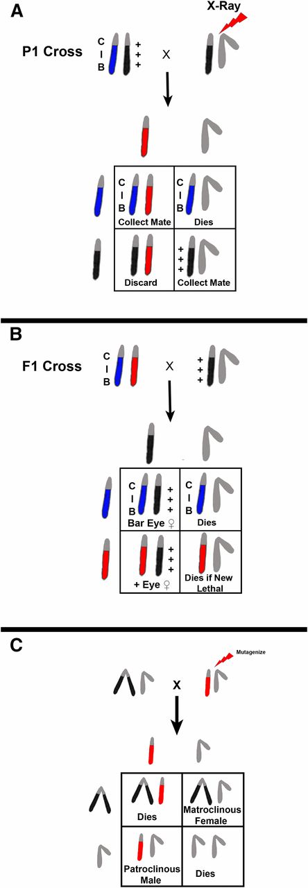
Schematic representation of Muller’s ClB screen for sex-linked lethals and/or visibles. (A) A cross of an X-ray-treated male to a ClB heterozygous female is shown. In the F1 progeny, ClB/X* female progeny are collected and mated to normal male siblings (B). The F2 progeny are scored for the presence of either non-Bar-eyed males or non-Bar-eyed males that have an altered phenotype. The limitation of this technique is that recovery of the chromosome with a newly-induced lethal mutation has to be accomplished from the X*/X+ sibling females, which have no convenient markers and can undergo free recombination between the two X chromosomes. This deficiency was overcome by development of better “balancer” chromosomes that are well-marked, viable, and fertile in males. If one is interested in recovering sex-linked visible or viable behavioral mutations, a generation can be saved by using attached X chromosomes. In this case, mutagenized males are mated to C(1)RM/Y females and the F1 progeny screened for changes (C). Each patroclinous progeny male will be the result of a single treated sperm and thousands of progeny can be easily surveyed.
If you want to screen for sex-linked visible or behavioral mutations that are viable and male fertile, it is possible to advantage of the attached X to save a generation, i.e., you can screen in the F1. Again, males are mutagenized, but in this case they are mated to C(1)RM/Y females. Each patroclinous male F1 progeny will be the product of a single mutagenized sperm and can potentially carry a newly-induced mutation. Obviously if the new lesion is lethal the male will not survive. However, if the new mutation falls into the aforementioned categories, you have saved a lot of single female crosses and can screen in bulk. This type of screen has been quite successful in the recovery of temperature-sensitive paralysis and flightless mutations (Grigliatti et al. 1972, 1973; Homyk et al. 1980).
Screening on the autosomes requires extra generations due to the fact that it is necessary to make the mutagenized chromosome homozygous and one does not have the advantage of the single X or hemizygous male. As in the sex-linked screens, males are mutagenized. To efficiently use the progeny produced, the males are mated to females heterozygous for two different balancer chromosomes. There are several of these combinations, e.g., CxD/TM3, available. In the F1, males carrying the mutagenized chromosome with either of the balancers are selected (Figure 15) and mated to several Bal#1/Bal#2 females similar to their mothers. Note that this F1 cross can also be done by mating single females carrying the mutagenized chromosome over either balancer and mating them back to males genotypically like the P1 female. In the F2 generation, males and females carrying the now cloned mutagenized chromosome over the same balancer are inbred. In the next F3 generation, the homozygous balancer animals die and the homozygous mutagenized progeny scored for visible changes or lethality. The lethal-bearing chromosome can then be recovered in the balancer sibling males and females and a self-selecting stock maintained. If the homozygous mutagenized progeny are viable, they can be tested for fertility or behavioral defects. The sterile lines in females can be caused by defects in ovary development per se or can act as maternal-effect steriles. If the homozygotes are fertile, their progeny can be tested for fertility in a screen for grand childless mutations. In both the fertility and grand childless screen, parallel cultures can be kept of the heterozygous balancer/mutagenized siblings to recover and maintain the induced lesion.
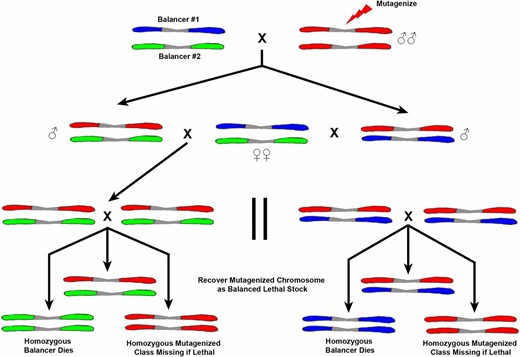
Schematic diagram showing one potential way to screen for mutations on the autosomes. Males are mutagenized with either irradiation or chemicals (red chromosomes) and mated to females carrying two different autosomal balancer chromosomes that are differentially marked (blue and green chromosomes). Single F1 males carrying a mutagenized red chromosome heterozygous with either balancer (blue or green) are mated to females similar to the P1 parent. In the F2 progeny, males and females carry one of the balancers (red and either green or blue) and a clone of the mutagenized red chromosome. The F3 progeny of this cross can be scored for a variety of mutant types. If the homozygous red animals are absent a lethal has been induced; if they are phenotypically changed a visible. In the case of lethality, the chromosome can be recovered in the heterozygous red over green or blue sibling progeny. This crossing scheme can be modified in a variety of ways and extended to recover steriles, maternal-effect, and grand childless mutations.
The screen described is a simple no-frills method for the recovery of autosomal mutations. There are a number of additions that can be used to eliminate some of the drudgery of doing this kind of screen. Temperature-sensitive mutations can be incorporated that selectively kill or sterilize males obviating the need to collect virgins, and dominant temperature-sensitive mutations in balancer chromosomes can be used to eliminate unwanted balancer-bearing progeny. Additionally, it is possible to use deficiency-bearing chromosomes to screen in specific regions of the autosomes and to eliminate the need of going to the F3 generation. In this case, the F1 balancer/mutagenized males or females are mated to deficiency/balancer animals of the opposite sex. The homozygous balancer progeny will die and the test generation mutagenized/deficiency scored for viability or phenotypic change. Again, the mutation-bearing chromosome can be recovered in the balancer-bearing siblings and a balanced stock recovered and maintained. A further discussion of additional embellishments to forward genetic screens can be found in St. Johnston (2002).
Mutagens
The efficient recovery of new mutations is of course dependent on the ability to raise the mutation rate above the low spontaneous rate. As noted above in the foundation years of Drosophila genetics, Muller found that X-rays served admirably for this purpose (Muller 1928). He was able to show that not only did irradiation produce lesions in individual genes (i.e., apparent point mutations), but that he could recover gross chromosomal rearrangements like those described above. Subsequent to this discovery, other types of ionizing radiation (α, β and γ) were tested and also found to cause mutations, albeit with variable efficiency. One of Muller’s goals in his mutation studies was to hopefully discover the nature of the gene, and while many of his predictions and hypotheses were interestingly prescient he never quite achieved his goal. A second attack on the nature of the gene, which again did not quite pan out, came from the use of chemicals as mutagens. The first of these was carried out by Auerbach with the demonstration that mustard gas is mutagenic in Drosophila (Auerbach and Robson 1946; Auerbach et al. 1947). Unfortunately, this work was done during WWII and the State Secrets Act did not allow her to publish until after the conclusion of the war. As in the case of radiation mutagenesis, additional chemicals were tested and a variety shown to be effective. Notable among these is EMS, which became one of the more popular (Lewis and Bacher 1968). Its popularity is associated with its ease of administration; it can be fed to adult males in a sugar solution combined with its high mutation rate. Feeding of a 0.25 M solution for overnight results in a nearly 50% mutation rate for sex-linked lethals, with many of the recovered chromosomes carrying > 1 hit (Ashburner et al. 2005). Lower doses of the chemical result in lower rates and fewer multiple hits. In addition to this alkylating agent, MMS and ENU have been shown to induce high rates of mutagenesis (Lee et al. 1989, 1990). The latter agent, while efficacious, has not garnered much favor due to its high toxicity and EMS has remained the go-to chemical mutagen.
A relatively novel class of mutagen was developed with the discovery of mobile genetic elements in the genome of Drosophila. Transposon mutagenesis has been a mainstay in the world of microbial genetics and has been used in flies in a similar fashion. One of the advantages to using transposable elements is that, when they insert into a target gene and cause its inactivation that gene is now tagged and can be identified molecularly by its association with the mobile element. Initially this type of mutagenesis was performed using a naturally occurring P-element (Ryder and Russell 2003; Hummel and Klämbt 2008). In its simplest form a genotype containing stable insertions of P-elements are crossed to strains expressing the transposase that will mobilize the target element. These animals are then crossed to recover new insertions and individual lines are screened for new mutations. This technique was then improved upon by the creation of P-element constructs that carried simple markers like the w+ and y+ genes. These were inserted into the genome transgenically, stabilized, and then mobilized as above. The phenotypic marker tags allow for the simple identification of the presence of the transposon and its easy genetic mapping. P-elements have the added virtue that when they excise they do so imprecisely. That is, they take with them adjacent genomic sequence leaving behind a deletion. Thus, remobilization of an insert can be used to create new lesions in genes targeted by the original insert. The P-element is not entirely random in its insertion and large collections of mobilized P inserts have shown that they favor landing in specific genes. Repeated mobilization in attempts to recover inserts in every gene have, thus, reached a point of diminishing returns and different transposable elements have been employed to increase the possibility of tagging every gene in the genome. Prominent among those being used are hobo, minos, and piggyback. These three elements have been used in a similar way as P and have been shown to produce a somewhat wider repertoire of hits, albeit not to the point of saturation. Also, imprecise excision characteristic of P is not seen in all of these elements, notably piggyback is a poor candidate for this technique. Similar to the simple w+ and y+ markers, other more elaborate constructs have been cloned into transposable elements and bee transgenically inserted into the genome. Subsequent mobilization of these have allowed the insertion and genome-wide distribution of regulatory elements [e.g., upstream activating sequences (UAS)], GFP protein tags, Flp-FRT and Cre-lox site-directed recombination system components, as well as ϕC31 integrase and attP landing sites to facilitate integration of plasmids containing attB sites to name just a few. All of this has conspired to dramatically increase the number of tools and reagents available to the fly researcher. An excellent and more detailed description of the above can be found in Venken and Bellen (2014) and need not be repeated here.
All of the technology cited in brief above has been significantly augmented by the advent of clustered regularly interspaced short palindromic repeats (CRISPR) genome editing and its adoption by the fly community (Bassett et al. 2013; Bassett and Liu 2014; Beumer and Carroll 2014). In its simplest form, it can and is being used to target specific genes and can potentially be used to inactivate every gene in the genome, protein coding and noncoding. Additionally, this technology can and is being used to do many of the same things that the modified transposable elements were designed to do: alter the regulatory properties of genes and tag their gene products. Some of the screening techniques cited above will be helpful in the recovery of these targeted-induced changes and the balancer chromosomes will be invaluable in establishing stable self-selecting stocks. We are entering an entirely new and very exciting era in the analyses of the Drosophila genome and its constituent parts.
Complementation and Mapping
While in theory a CRISPR-induced mutation should have its genomic location known very precisely, the potential for off-target effects would seem to dictate that additional evidence for the location of any associated defect be confirmed genetically. Additionally, any new mutation recovered by more traditional screening methods needs to be located or mapped. There are several methods used in flies; the easiest is simple complementation with existing mutations. The mapping generally requires a set of preexisting well-characterized alleles, hopefully with a known genomic location. Given this, one simply crosses the unknown mutations to this preexisting set and failure of complementation immediately identifies and localizes the new lesion. However, as noted above, there are many more unlocalized mutations than those mapped to the genome so this technique is of limited utility beyond simply associating mutations into functional groups, which admittedly is not a bad thing. A second method is recombination or meiotic mapping. In general, the new mutation is localized to a chromosome and preferably a chromosome arm by its pattern of segregation or this general location is known by virtue of the nature of the screen that was performed (e.g., sex-linked vs. autosomal). Known visible markers are then selected that are appropriate for the new mutation. The BDSC has a set of nicely marked chromosomes that can be used for this purpose (http://flystocks.bio.indiana.edu/Browse/misc-browse/mapping.php). If the new mutation is sex-linked it is crossed to the mapping chromosome and heterozygous females recovered. These females are then backcrossed to males from the mapping stock and the resultant male progeny scored for exchange events. If the new mutation is lethal, the markers most tightly linked to it will show altered ratios (nonreciprocally) of recovery in the male exchange progeny and the proximity of the lethal to the markers determined. On the autosomes, things are bit more complicated and using markers that are dominant can simplify matters. In this case, the new mutation is crossed to the marker stock and heterozygous females recovered. These are then mated to the males from the new mutant stock. Similar to the sex-linked example, the dominant marker most tightly linked to a lethal will show an altered ratio in the exchange progeny. Since preexisting dominant mutations are not available for large regions of the autosomes, mapping using these is of necessity approximate. This problem has been overcome by the development of a series of P-element insertions marked with w+ that span all of the major chromosome arms (Zhai et al. 2003). These insertions have known or estimated recombination map positions and the added virtue of having been mapped molecularly, and thus have precisely known molecular genomic coordinates. Stocks of these are available from the BDSC (http://flystocks.bio.indiana.edu/Browse/misc-browse/Baylor-kits.php). If the new mutation can be placed or is in a w− background, the w+ tag in the P insert can be used as a dominant marker. Animals from the mapping stock are crossed to the new mutation, heterozygous females recovered, and backcrossed to males from the mutant stock. Again, proximity of the lethal and the w+ marker can be gauged by the relative recovery of red- and white-eyed progeny. Maps showing the relative positions (meiotic and cytological) of the markers in the various mapping stocks at the BDSC are shown in Figure 16.
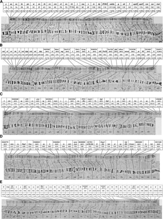
Polytene X (A), second (B and C), and third (D and E) chromosome maps after Bridges and Lefevre showing the relative map positions of markers useful for recombination mapping. Stocks containing different combinations of these markers are available at the Bloomington Drosophila Stock Center (http://flystocks.bio.indiana.edu/Browse/misc-browse/mapping.php and http://flystocks.bio.indiana.edu/Browse/misc-browse/Baylor-kits.php). The tables above the chromosomes list the gene symbols (top row), numbered and letter cytological location (middle row), and approximate recombination map position in centi-Morgans of each marker. The lines connecting the tables to the chromosome arms indicate the approximate cytological position of the markers. The markers include lesions that are associated with visible phenotypic changes as well as transgenic insertions carrying the w+ gene.
As noted above, a second method for mapping is what I will refer to as cytological. A set of well-characterized deficiencies with known molecular endpoints has been assembled by the BDSC into what is referred to as the “Deficiency Kit” (http://flystocks.bio.indiana.edu/Browse/df/dfkit.php). Animals from the new mutation stock are crossed to those from the kit and the progeny scored for phenotype, or in the case of lethals for simple presence or absence. The exposure of the new mutation by a deficiency from the kit immediately reveals the molecular domain in which the mapped lesion lies. The BDSC also has additional deletions that can be used to subdivide the interval defined by the kit deletion and can localize many genes to seven or fewer annotated loci. For genes on the X, things are a bit more complicated but not insurmountable. If the new mutation is lethal or male sterile, males carrying the lesion cannot be recovered or used in a cross, and in most cases the deficiency mapping kit stocks carry the deletions only in females. This problem has been overcome by the existence of the Y-linked (http://flystocks.bio.indiana.edu/Browse/dp/Dp_bsc.php) (Cook et al. 2010) and transgenically-produced (http://flystocks.bio.indiana.edu/Browse/dp/Dp_tns_X.php) duplication-bearing stocks (Venken et al. 2010). The larger Y-linked duplications can be used to recover males carrying the new mutation balanced by the duplicated material on the Y. Since the molecular coordinates of the duplication are known, the smaller transgenic duplications in the same interval can be used to subdivide the larger region in a conceptually similar way to autosomal deficiency mapping. The molecular endpoints of the smaller duplications are known so coverage maps locate the new lesion more precisely. Now that males are available, these can be used in crosses to females taken from the BDSC collection to even more precisely localize the new lesion.
Finally, it is possible to molecularly map mutations by sequencing. Sequencing technology has improved and costs reduced so that it is feasible to do this at the whole-genome level. This of course requires that the new mutation has been induced in a rigorously-established isogenic background and that the mutagenesis does not create large numbers of second-site lesions. Since these two criteria are seldom met, it is preferable to have some way to constrain the region of the genome to be sequenced in the search for the causative mutational event. Using either the recombination mapping or preferably the deletion/duplication mapping described above is an advised, if not mandatory, first step. Again, this methodology is described in detail in Venken and Bellen (2014).
Classification of Mutation Types
Muller (1932) coined the terms Amorph, Hypomorph, Hypermorph, Antimorph, and Neomorph to classify mutations. This cataloging was based on the genetic and dose-response behavior of the mutations that the Drosophila community had been collecting since 1910, augmented by the large number of mutations he had recovered using X-ray mutagenesis.
An Amorphic mutation is one that causes a complete loss-of-function. These lesions are also often referred to as null. Functionally, an amorphic mutation shows an identical phenotype when in homozygotes and when hemizygous, i.e., mutation/deficiency. Amorphs are commonly recessive; however, they can also show a dominant phenotype if the gene product is haploinsufficient, i.e., its product is required in two copies. In Drosophila, the Minutes are classic examples of just such an amorphic dominant.
Hypomorphic mutations are associated with only a partial loss-of-function. Functionally, a hypomorph shows a more severe phenotype when hemizygous, i.e., mutation/deficiency, than is seen in the homozygous condition. Like amorphs they are usually recessive. Studies of a hypomorphic series of lesions in a gene, i.e., using a graded series of phenotypes from less to more severe, can be instructive in deducing a gene’s function.
The remaining three categories are often referred to collectively as gain-of-function mutations and are generally dominant to their corresponding wild-type allele. This can be associated with either a change in the functionality of the gene product, a change in the level of expression, or in the regulation of the expression pattern temporally or spatially.
Hypermorphic mutations are associated with an increase in normal gene function. This can be caused by an upregulation of gene expression or the simple duplication of a gene. Functionally, the phenotype of a hypermorph is made more extreme by increasing the number of wild-type copies, e.g., using a duplication of the gene, and is ameliorated by reducing the dose, e.g., using a deletion.
Antimorphs are generally dominant and encode a gene product that acts antagonistically to the wild-type allele. Antimorphs are also referred to as dominant negatives. An increase in wild-type gene dosage using a duplication reduces the phenotypic severity of an antimorph. This type of mutation is often associated with proteins that act as dimers or higher-order multimers. When these defective peptides are incorporated into the multimer their presence serves to inactivate the complex. Their behavior as homozygotes is generally to cause lethality.
Neomorphic mutations are, like antimorphs, dominant gain-of-function alleles. They are generally associated with ectopic expression of a normal gene product in a new temporal or spatial pattern or the encoding a protein product that has gained some new functionality. Unlike the antimorph, increasing wild-type gene dose with a duplication has little effect on the mutant phenotype and it is this genetic property that serves to distinguish the neomorph from the antimorph. Making an neomorph hemizygous is generally associated with lethality, but only if the wild-type functionality of the allele has been compromised by the change that results in the ectopic pattern of expression.
The Muller categories were based on the genetic and dosage properties of recovered mutations but it should be remembered that those classifications, while valuable, were made prior to the molecular characterization of the gene. Thus, we can now classify mutations at that level as well: single-base pair changes can result in nonsense or missense mutation. Nonsense mutations are associated with the production of stop codons and can result in the production of truncated protein products or no product at all through nonsense-mediated decay. Missense mutations are again single-base pair changes in coding sequences that result in an altered amino acid. This type of change can have minor or catastrophic effects on encoded protein function. These types of changes generally fall into Muller’s amorph or hypomorph categories; however, these single-codon changes can also result in antimorphic or neomorphic types if the lesions are associated with critical amino acid changes in or truncation deletions of functional protein motifs. In Humans, Machado Joseph disease and Huntington’s disease are associated with polyQ tracks and these have been modeled in Drosophila (Xu et al. 2015; Lewis and Smith 2016; Krench and Littleton 2017).
If single base pairs are either inserted or deleted from a coding exon the change will result in frameshift mutations. These changes are associated with an altered coding potential from the point of the deletion/insertion to the end of the open reading frame. Often, the downstream effect is the production of an in-frame stop codon and the production of a highly altered truncated peptide. If the insertion or deletion occurs early in the open reading frame, these lesions are most often amorphic and null.
End Note
If you have made it this far, I hope you have found some useful information in the above. When I began this writing, I had a rather different product in mind. Based on the large number of methods papers and books available, I ended up with a more historical view rather than simply repeating much of what is presented in them (Greenspan 2004; Roote and Prokop 2013). What was produced is a short introduction to the Drosophila genome and its contents, followed by a bit of what my friend and colleague John Lucchesi has referred to as “Chromosome Mechanics” (Lucchesi 1994). Given the wealth of information on this topic and the enormous contributions made by Drosophila, its adherents, and champions, I have of necessity only scratched the surface. My segment on genetic screens was colored by the advent of CRISPR and the way that technology has spread through the scientific community, including those who work on flies. Describing screens, thus, has largely become part of the history of genetics and genomics. While there is still a role for screens that seek to find mutations that produce specific phenotypes and I firmly believe there will still be surprises there, knocking out a specific gene’s function has now turned into a rather mechanical exercise. While powerful and likely to provide an enormous volume of information, I like to remember the “old days” with some fondness. We knew a lot less and doing genetics was a very conceptual science. It was a long way from genotype-to-phenotype. Nevertheless, that in no way diminished our joy and great excitement with every new discovery and insight.
Footnotes
This chapter in FlyBook is dedicated to the memory of my dear friend and colleague Dr. William Martin Gelbart. Bill’s contributions to the field of Genetics in general and to Drosophila specifically were numerous and significant. We are all the better for his commitment to our community and the less with his passing.
Communicating editor: H. J. Bellen
