


Abstract
Adaptation to environmental stress is critical for long-term species persistence. With climate change and other anthropogenic stressors compounding natural selective pressures, understanding the nature of adaptation is as important as ever in evolutionary biology. In particular, the number of alternative molecular trajectories available for an organism to reach the same adaptive phenotype remains poorly understood. Here, we investigate this issue in a set of replicated Drosophila melanogaster lines selected for increased desiccation resistance—a classical physiological trait that has been closely linked to Drosophila species distributions. We used pooled whole-genome sequencing (Pool-Seq) to compare the genetic basis of their selection responses, using a matching set of replicated control lines for characterizing laboratory (lab-)adaptation, as well as the original base population. The ratio of effective population size to census size was high over the 21 generations of the experiment at 0.52–0.88 for all selected and control lines. While selected SNPs in replicates of the same treatment (desiccation-selection or lab-adaptation) tended to change frequency in the same direction, suggesting some commonality in the selection response, candidate SNP and gene lists often differed among replicates. Three of the five desiccation-selection replicates showed significant overlap at the gene and network level. All five replicates showed enrichment for ovary-expressed genes, suggesting maternal effects on the selected trait. Divergence between pairs of replicate lines for desiccation-candidate SNPs was greater than between pairs of control lines. This difference also far exceeded the divergence between pairs of replicate lines for neutral SNPs. Overall, while there was overlap in the direction of allele frequency changes and the network and functional categories affected by desiccation selection, replicates showed unique responses at all levels, likely reflecting hitchhiking effects, and highlighting the challenges in identifying candidate genes from these types of experiments when traits are likely to be polygenic.
UNDERSTANDING how adaptation proceeds in a population is important for predicting natural responses to impending stress that will challenge the adaptive potential of many species. Climate stress is a timely example: our ability to predict and respond to climate change effects on natural populations requires relevant models of how evolution proceeds, backed up by empirical evidence.
Aridity is one climate-imposed stress likely to increase in parts of the world as climate change proceeds. Many areas that currently experience reasonable rainfall are projected to become drier over the coming decades (Dai 2012), and some are already showing significant reductions in rainfall (e.g., southwestern Australia: Delworth and Zeng 2014). Dry conditions typically impose water balance stress on organisms, and, when there is no behavioral escape possible, the only opportunities for survival are tolerance or adaptation (Franks and Hoffmann 2012).
The potential for adaptation to desiccation stress varies greatly among species. Many plants show evidence of both plastic and adaptive responses to aridity (Des Marais and Juenger 2010; Byrne et al. 2013; Juenger 2013). This has been harnessed in crop breeding through artificial selection for efficient water use, though increasing aridity will likely still challenge agriculture (Qureshi et al. 2013). In animals, there is extensive knowledge from Drosophila melanogaster about the potential for adaptation to numerous climate stresses (Hoffmann et al. 2003, 2005; Franks and Hoffmann 2012), and artificial selection experiments have demonstrated this species can readily evolve higher desiccation tolerance (Hoffmann and Parsons 1989a; Hoffmann et al. 2003) with reported heritabilities of around 60% (Hoffmann and Parsons 1989b; Kellermann et al. 2009). However, some related species respond quite differently when faced with dry conditions. The Australian rainforest endemics D. birchii and D. bunnanda both have zero, or very low, adaptive potential under extreme desiccation stress (Hoffmann et al. 2003; Kellermann et al. 2009), although they do show significant heritability under more moderate levels of stress (van Heerwaarden and Sgro 2014). The widespread species D. melanogaster and D. serrata, however, are able to adapt even to the more severe levels of desiccation (Hoffmann and Parsons 1989b; Blows and Hoffmann 1993).
Numerous subphenotypes have been linked to desiccation resistance in drosophilids, including cuticle composition (Rajpurohit et al. 2013); reduced water loss rate (Hoffmann and Parsons 1993; Gibbs et al. 2003); metabolic rate; glycogen, lipid and/or carbohydrate storage (Hoffmann and Harshman 1999); and sensing and signaling pathways (Telonis-Scott et al. 2012, 2016). Identifying the specific loci involved in adaptation to stress offers possibilities for assessing the generality of stress adaptation, both within, and across, species (Franks and Hoffmann 2012; Byrne et al. 2013). Knowing to what extent stress adaptation proceeds from predictable genes, gene families, or regulatory network modules will aid in predicting adaptive capacity for species in which experimental manipulation is not possible. Further to this, assessing how a population adapts to a stress at the genomic level has implications for population size dynamics and connectivity, which affect population resilience to other stresses and future adaptive capacity (Willi and Hoffmann 2009; Hoffmann and Sgrò 2011).
This paper deals with the use of selection experiments to understand how, and where, adaptation proceeds across the genome, how repeatable it is, and how selection influences divergence or convergence across the genome. An evolve-and-resequence (E&R) approach—where replicate lines from a common genetic background are characterized for genomic variation after a period of selection—is useful for studying these questions as a step toward understanding the generality of responses to climate stress. In the past, this approach has been used in sexual species to investigate genotype-phenotype associations for lab-adaptation (Teotónio et al. 2009; Burke et al. 2010; Simões et al. 2010; Orozco-terWengel et al. 2012; Santos et al. 2012; Burke et al. 2014), adaptation to diet (Reed et al. 2014), and thermal adaptation (Tobler et al. 2013; Franssen et al. 2014), as well as for investigating the dynamics of adaptation across the genome with phenotype as a secondary consideration (Burke et al. 2014). How many loci respond to selection, and how large an effect they have on the phenotype, are important parameters to consider because of their implications for adaptive potential, genetic diversity, and divergence at the population level. It has been suggested that strong selection will favor large-effect alleles (Orr 2010) but these may also carry large negative pleiotropic consequences.
Many Drosophila E&R studies have identified numerous small-effect loci responding to selection (Teotónio et al. 2009; Burke et al. 2010; Turner et al. 2011; Turner and Miller 2012; Orozco-terWengel et al. 2012), but some authors have suggested this may be an artifact of experimental designs that have limited power to detect true causative loci, particularly because of hitchhiking effects (Kofler and Schlötterer 2013; Tobler et al. 2013; Baldwin-Brown et al. 2014). Another problem with E&R experiments is the potential for experimental populations to adapt to laboratory conditions alongside the actual selective pressure of interest, which can be difficult to disentangle (Harshman and Hoffmann 2000; Matos et al. 2000; Santos et al. 2012). In this experiment we attempt to increase power by maintaining moderate effective population size, and by identifying lab-adaptation candidate loci in replicated control lines, and removing them from the candidate loci sets identified for desiccation resistance.
Understanding to what extent adaptation to climate stress is repeatable also has implications for conservation management under climate change. If a relevant trait has low evolutionary repeatability, perhaps adaptive potential is simply a function of the level of starting genetic variation in the population; on the other hand, if evolution is reasonably repeatable, a population’s adaptive capacity will rely more heavily on the presence of specific variants (or the possibility that these will enter the population via gene flow). Results vary as to the extent to which experimental evolution is repeatable. Notably, the scope, limitations, and potential biases of E&R experiments in asexual (typically microbial) and sexual (typically Drosophila) species are different (reviewed in Burke 2012). Many studies in asexual taxa (e.g., Lohbeck et al. 2012; Tenaillon et al. 2012; Lang et al. 2013) have found little similarity among the loci involved in replicate lines from the same starting population, and many studies in sexual taxa have found evidence of parallel evolution (Teotónio et al. 2009; Burke et al. 2010, 2014; Reed et al. 2014). At a broader evolutionary scale, there are numerous examples of the same SNP, gene or genetic pathway being “reused” in widely divergent species in a similar evolutionary context, but ascertainment bias may play a part in this (Elmer and Meyer 2011; Martin and Orgogozo 2013), and there are also numerous examples of related taxa with different genetic paths to the same phenotype (Arendt and Reznick 2008; Elmer and Meyer 2011; Martin and Orgogozo 2013; Stern 2013). Clearly, it is not currently possible to generalize about the repeatability of evolution (Martin and Orgogozo 2013), and it is likely that it will vary greatly depending on the trait and species in question (Lobkovsky and Koonin 2012).
In this study, we focus on understanding the genetic basis and repeatability of evolution in response to desiccation stress. Specifically, we address the questions:
Which genomic regions are involved in desiccation stress response?
Which genomic regions are involved in lab-adaptation?
Are there consistent stress-responsive and lab-adaptation genomic landscapes among the replicate lines, and, if not, is the approach used able to establish similarity?
Is there a broader-scale signature of consistent selection response at the protein interaction network level, and/or the functional level?
Does selection increase or decrease divergence among replicate lines at the genomic level—and if so, to what extent is this due to the selection process rather than to changes in effective population size?
To tackle these questions, we use five replicate Drosophila lines derived from the same field-collected mass-bred population, selected for desiccation tolerance for 13 generations and compared to five control lines maintained under the same conditions and at the same population size.
Materials and Methods
Fly cultures
All cultures were held at constant 19°, under 12:12 hr light:dark cycle in 250 ml bottles containing laboratory medium composed of dextrose (7.5% w/v), cornmeal (7.3% w/v), inactive yeast (3.5% w/v), soy flour (2% w/v), agar (0.6% w/v), 4-methyl 4-hydroxybenzoate (1.6%), and acid mix (1.4% 10:1 propionic acid:orthophosphoric acid). The experimental flies were reared under controlled density conditions by removing parents from the bottles after 48 hr of oviposition.
Selection regime
The desiccation-selected and control lines were founded from D. melanogaster collected at Templestowe, a suburb in Melbourne, Australia, in May 2012. The offspring of 60 field-collected females (i.e., >240 haploid genome equivalents, depending on multiple mating; Griffiths et al. 1982) were pooled and mass-bred for two generations in the laboratory prior to the first selection. From the resulting ∼11,200 generation 0 flies, 200 were set aside for sequencing as the generation 0 mass-bred representatives; 1000 flies were set aside to found the five replicate control lines (see below). The remaining 10,000 were exposed to desiccation stress as follows: 5000 virgin females and males were separated by sex under light CO2 anesthesia, and held in separate vials according to sex, at a density of 25 individuals per vial. The selection experiments for desiccation resistance were done separately for both sexes at 4–8 days post eclosion. Flies were desiccated in groups of 25 in glass vials topped with gauze in sealed glass tanks containing silica desiccant (relative humidity <10%) at 25° until ∼90% of the flies had died, noting the time point at which this occurred (LT90). The surviving 10% of flies were collected, and randomly allocated into five replicate lines comprising 100–110 flies of each sex (200–210 in total) per replicate. For each of the following selected generations, 1000 females and 1000 males per line were stressed, and the 10% most desiccation-resistant adults (100–110 of each sex, 200–210 in total) were kept as parents for the next generation. The control lines were established and maintained in the same manner as the desiccation-resistant lines, but these lines were not exposed to any treatment. They were maintained at equivalent population sizes as the selected lines, and 100 flies of each sex were randomly chosen to found each new generation. Flies were selected for desiccation resistance every generation until generation eight, and every second generation thereafter until generation 21. The desiccation-resistant selected lines will be referred to as “desiccation replicates” D1–D5, and the control lines as “control replicates” C1–C5.
Desiccation selection response assay
All lines were assessed for desiccation resistance after eight generations of selection. The desiccation assay was performed separately on each sex, and after two generations of relaxation to ensure that any differences found in the subsequent experiments were genetic rather than due to cross-generation effects (Schiffer et al. 2013). Flies were sexed under light CO2 anesthesia and held in separate vials according to sex, and the desiccation assays were performed on 4- to 6-day-old flies. Flies were desiccated as described above, and scored at hourly intervals until 100% mortality was reached (LT100). LT90 was used for the statistical analyses.
Desiccation resistance was analyzed using mixed-model analysis of variance using the MIXED procedure and Kenward-Roger degrees of freedom method (Littell et al. 2006) in SAS software v9.3 (SAS Institute, Cary, NC). Models were run separately for each sex. Selection regime was included as a fixed factor, and line (nested under selection regime) as a random factor.
Fly sampling and DNA sequencing
At generation 0 (the mass-bred) and after 13 generations of selection, the flies were frozen after they had laid eggs to start the next generation. Fifty individuals from each line (25 females and 25 males) were randomly chosen, and their heads removed for pooled DNA extraction, except for the generation 0 sample, where 200 individuals (100 females and 100 males) were used in order to be able to detect alleles that were rare in the starting population. In this case, the 200 individuals were processed in four pools of 50 so as to be comparable to the other samples. Samples were labeled MB1–4 (mass bred), C1.13 (control line 1, generation 13 of selection) through to D5.13 (desiccation line 5, generation 13 of selection). Each pool of 50 heads was ground in Qiagen buffer ATL using a plastic pestle, and DNA was then extracted following the Qiagen DNeasy Blood & Tissue kit protocol (Qiagen, Hilden, Germany). The DNA was fragmented and libraries were prepared starting from 1 µg genomic DNA, at the UPC Genome Core, University of Southern California. In total, nine lanes of Illumina 100 paired-end sequencing were performed. Initially, eight lanes were sequenced, with each of the 24 libraries barcoded and pooled in equimolar amounts in each lane. Some libraries produced low read numbers, however, and these were repooled and resequenced in a further lane. This was repeated twice until all libraries appeared to have sufficient coverage (minimum: ∼31 × 106 paired-end reads) for downstream comparison. Raw reads are available from the NCBI Sequence Read Archive as BioSamples SAMN04361549 to SAMN04361559 in BioProject PRJNA306702.
Bioinformatic data processing
Initial data processing was performed at the Victorian Life Science Computation Initiative (VLSCI), using a custom version (Griffin 2016a) of the Rubra pipeline (Pope et al. 2013) available at https://doi.org/10.5281/zenodo.166394. Raw reads were checked for quality using FastQC (Andrews 2010), and trimmed with Trimmomatic v 0.30 (Lohse et al. 2012) using the following parameters: LEADING:30 TRAILING:30 SLIDINGWINDOW:10:25 MINLEN:40, removing adapter sequences, allowing zero seed mismatches, a palindrome clip threshold of 30, and a simple clip threshold of 30.
Trimmed reads were then aligned to the reference genome, D. melanogaster r6.01, with the bwa v6.2 (Li and Durbin 2009) aln command, and settings “-t 8 -n 0.01 -o 2 -d 12 -e 12 -l 150” to maximize the mapping of genetically diverged reads to the reference genome. The resulting files were converted to sorted .bam format by way of the bwa sampe and Picard v 1.96 (Broad Institute 2014) SortSam tools. At this point, .bam files belonging to the same pool of flies, but coming from different sequencing lanes, were merged. Duplicate reads were removed with Picard MarkDuplicates, and all files were used as input to the GATK v2.6-5 (DePristo et al. 2011) tools RealignTargetCreator and IndelRealigner in order to perform local realignment around indels, which can otherwise cause false SNP calls. The four files for the four mass-bred (generation 0) pools were then downsampled to have the same number of total reads, and merged into a single “MB” file to represent the entire mass bred pool as a whole.
A repeat-masked version of the r6.01 reference genome was created with RepeatMasker v4.0.3 (Smit et al. 2013–2015), and the settings “-s -no_is -nolow -norna -pa 8 -div 50 -e rmblast.” The repeat library contained all annotated transposons from D. melanogaster, including shared ancestral sequences (Flybase release r5.57), and all repetitive elements from Repbase Update release v19.04 for D. melanogaster (Jurka et al. 2005). The Samtools v 0.1.19 (Li et al. 2009) mpileup command was used for initial SNP calling of all 11 pools, using the repeat-masked reference genome and the settings “-q 20 -d 1000000 -R -A –B.” This was performed for each file individually, for all files together, and for MB vs. each of the other samples (see below). Each pileup file was converted to sync format with the mpileup2sync.jar tool in Popoolation2 (Kofler et al. 2011).
Candidate SNP identification
The first step in candidate SNP identification involved finding SNPs whose frequencies had changed significantly between the mass-bred and generation 13 pool for each of the control and desiccation replicates. Fisher’s exact test (Fisher 1922) was performed for each replicate on the sync file containing the mass-bred and generation 13 data. It was run in Popoolation2, with the following settings: minimum count of the minor allele: three reads; no minimum coverage depth; maximum coverage: 10,000 reads; suppressing output of noninformative (non-SNP) loci. These settings had previous been ascertained to produce comparable numbers of SNPs across all experimental line pools despite varying coverage depth (Supplemental Material, Figure S1). We applied a Bonferroni-corrected α = 1 × 10⁻⁶ calculated for each replicate to adjust for multiple comparisons (Table S1).
We also applied the likelihood ratio test suggested by Lynch et al. (2014), as well as a significance threshold based on the 95% frequency interval around final allele frequency expected due to genetic drift alone (see File S1 for details). These tests were implemented in R v3.1.0 (R Core Team 2014). For each replicate, our final set of loci that were significantly differentiated between the mass-bred and generation 13 pools comprised those that fit all three conditions: those with a Fisher’s exact test P-value lower than the Bonferroni-adjusted threshold; those with a P-value from the Lynch et al. (2014) likelihood ratio test below the Bonferroni-adjusted threshold; and those whose frequency change exceeded the 95% confidence interval bounding the simulated frequency change under drift alone. In practice, performance in the Fisher’s exact test was the most conservative of these three conditions, and was the limiting factor in the majority of cases for judging whether or not a SNP was a candidate.
SNP location and effect annotation
We tested whether known inversions were involved in genomic responses to selection. We examined allele frequencies in our mass-bred and generation 13 pools at SNPs diagnostic for the inversions In3R(P) (Anderson et al. 2005; Kapun et al. 2014), In(2L)t (Andolfatto et al. 1999; Kapun et al. 2014), In(2R)Ns, In(3L)P, In(3R)C, In(3R)K, and In(3R)Mo (Kapun et al. 2014).
To further investigate the chromosomal arrangement of highly differentiated regions, we visualized the proportion of SNPs attaining significant differentiation in chromosome windows of 100 kbp and 1 Mbp (Figure S2). We then performed two tests to explore whether these highly differentiated regions represented haplotypes that were present at low frequency in the starting population, and might have been lost in some replicates, but swept to high frequency in others. First, for each 100 kbp window, we calculated the proportion of low-frequency SNPs, identified as those SNPs with “selected” alleles present at generation 0 frequency below 0.1. We applied a linear model at the chromosome level per replicate line to test whether the proportion of low-frequency SNPs was related to the proportion of significantly differentiated SNPs (both including and excluding windows with no significantly differentiated SNPs). Second, we identified all “enriched” 100 kbp windows where the proportion of significantly differentiated SNPs was in the 80th percentile (calculated across the whole genome, after excluding windows with no significant SNPs). Where two or more such windows occurred within 1 Mbp of each other, we marked the entire intervening region as a region enriched in significant SNPs (see Figure S2). This allowed regions to vary in size, representing potential long-distance hitchhiking effects. We then compared two logistic regression models, where “enriched” vs. “nonenriched” status was the response variable, explained in model 1 solely by the overall proportion of low-frequency SNPs, and explained in model 2 by both the overall proportion of low-frequency SNPs, and the proportion of significantly differentiated SNPs that were at a low frequency. An analysis of variance on the two models allowed us to test whether the proportion of significant SNPs that were low-frequency significantly improved predictions of “enriched” status. This test was performed at the whole-genome level per replicate line.
The list of candidate SNPs was converted to vcf format with a custom R script convert_sync_to_vcf.R (available at https://doi.org/10.5281/zenodo.166392; Griffin 2016b). Where both the major and minor alleles differed from the reference genome, the “reference allele” was set as the allele that decreased in frequency from the mass-bred to the generation 13 pool. The “alternate allele” was always set as the allele that increased in frequency. The genomic features in which the candidate SNPs occurred were annotated using snpEff v4.0, first creating a database from the D. melanogaster v6.01 genome annotation, with the default approach (Cingolani et al. 2012). Default parameters were used for the annotation, with the “−ud 1000” parameter annotating any SNP within 1000 bp of a gene to that gene. We then tested for over or underenrichment of feature types using χ2 tests, comparing the number of features from all SNPs detected in the mass-bred generation 13 with the number of features found in the list of candidate SNPs for each replicate (Fabian et al. 2012). We separately extracted SNPs predicted to have a high impact on protein function (a stop codon loss or gain, or a splice site variant) for further investigation.
Overlap among candidate SNP lists was quantified, and the significance of overlap was tested as follows. The row positions of the significant SNPs were identified in the snpEff output file. To resample, the same number of rows was chosen by shunting positions forward by a random integer (between 1 and the length of the file), wrapping around to the start of the file. This was similar to the approach used by Nordborg et al. (2005), and retained the effect of any linkage disequilibrium (LD) between SNPs without having to characterize LD extent, which is difficult in pooled samples (Franssen et al. 2014). Overlap (number of SNPs in common) was calculated among all pairs of SNP lists in each simulation. The entire simulation was performed 1000 times. The distribution of simulated overlap was plotted as a histogram to which the observed overlap could be compared.
Consistency of allele frequency change
As a complementary approach to the overlap test described above, we tested the hypothesis that selection favored the same set of alleles in each experimental replicate using allele frequency change direction. We reasoned that, if selection favored a common set of alleles, we would expect desiccation-selected allele frequencies generally to change in the same direction over time across the desiccation replicates, but not across the controls. We extracted the set of significantly differentiated SNPs for each gen0–gen13 comparison of a desiccation replicate, excluding SNPs from the desiccation-replicate sets that occurred within 1000 bp of a putative lab-adaptation gene. A two-sided t-test was then used to test whether the mean proportion of loci changing in the same direction (excluding the focal line itself) differed between control and desiccation replicates. In this test, the fly lines were the data points, not the SNPs. This was repeated by treating each of the five desiccation replicates as focal lines in turn. For the control replicates, we followed the same procedure, extracting allele frequencies for candidate SNPs in all other replicates, and calculating the proportion of loci in each replicate that changed in the same direction as they did in the focal control line. We also used these results in an overall ANOVA to test whether the proportion of loci changing in the same direction as in the focal sample differed between the control or desiccation replicates.
Candidate gene and eQTL/veQTL identification, and gene list overlap testing
For each replicate, a gene list was extracted from the snpEff output file, first using snpSift (Cingolani et al. 2012), and then parsing gene names in R to include all unique names (parse_and_convert_gene_names.R script, available at https://doi.org/10.5281/zenodo.166392; Griffin 2016b). If a SNP mapped to multiple genes, all gene names were included. Any gene occurring in one or more control replicate was considered a putative lab-adaptation gene, and excluded from the desiccation replicates for all further analysis.
To test whether longer genes were more likely to be detected in our overlapping gene lists, we examined the relationship between gene length and frequency of gene appearance in the simulated lists, and compared it to the distribution of gene length in the observed list. For the simulated SNP lists, the resampled snpEff file rows (see above) were then parsed as before to include all unique gene names. Overlap was calculated among all combinations of simulated gene lists (removing genes occurring in any C-replicate in that simulation from any simulated D-replicate list). In this analysis, gene length was extended to include the 1000 bp upstream and downstream regions because this was the setting used previously for SNP annotation. The function of candidate genes occurring in multiple replicates from this and other analyses was investigated in FlyBase (Santos et al. 2015). We investigated whether SNPs mapping to multiple genes were driving patterns of overlap (see File S1 for details).
We also tested whether the candidate SNP sets were enriched in SNPs known to be eQTLs or veQTLs (i.e., SNPs influencing the expression level, or expression variance, of a gene). We checked each candidate SNP set in turn against a list of all eQTL/veQTL SNPs identified at the FDR <0.20 level by Huang et al. (2015). We then compared the observed number of candidate eQTL/veQTL SNPs to the null distribution provided by the 1000 simulated SNP lists described above. In this test, the full candidate SNP sets were used for the desiccation replicates without removing putative lab-adaptation candidates. We also identified the unique genes predicted as targets of each set of candidate eQTL/veQTL SNPs, and tested whether the number of targeted genes occurring across replicates was higher than expected by chance.
Analysis of drift, selection, and effective population size
Additionally, pairwise FST was calculated across 100,000 bp windows among each pair of desiccation or control replicates with the fst-sliding.pl script in Popoolation2 (Kofler et al. 2011), with the options “--min-covered-fraction 0.0 --suppress-noninformative --window-size 100000 --step-size 100000 --min-count 3 --min-coverage 4 --max-coverage 100000”.
Gene ontology (GO), developmental stage and body part category enrichment
We investigated whether the gene lists were enriched in known function, or enriched in genes expressed in particular developmental stages or organs. These analyses used Gowinda v1.12 (Kofler and Schlötterer 2012) run in gene mode, with 100,000 simulations, and assigning SNPs to genes based on their position, with the option “—gene-definition updownstream1000” annotating SNPs within 1000 bp of a gene. This program accounts for gene length. For the desiccation-selected replicates, the “significant SNP” list was first edited to exclude any SNP that occurred within 1000 bp of a putative lab-adaptation gene.
The GO annotations were taken from FuncAssociate 2 (Berriz et al. 2009), as recommended by the Gowinda authors (Kofler and Schlötterer 2012). The developmental stage and body part enrichment annotations were created as follows. Gene expression “pmax” data from Murali et al. (2014) was kindly provided by the authors. This data contained expression levels for all genes assayed in FlyAtlas (Chintapalli et al. 2007) and modENCODE (Graveley et al. 2011) scaled to a percentage of the maximum expression level observed in any category. If a gene was expressed at 75% or more of its maximum level in a given category, it was added to the gene list for that category. These category gene lists were then used as input to Gowinda with the same settings as for the GO enrichment tests. This analysis was repeated using 50 and 90% maximum expression as alternative category membership thresholds.
Protein–protein interaction network building and overlap testing
Gene names were converted to FBgn format using a custom R script parse_and_convert_gene_names.R (available at https://doi.org/10.5281/zenodo.166392; Griffin 2016b) and name-to-FBgn mappings from the snpEff “genes” output file. In a few cases, gene names extracted from the snpEff were in the format “Exon_chr_start_end”: the appropriate annotations were manually added using Flybase.
A “background” Drosophila protein-protein interaction (PPI) network was built with the igraph R package (Csardi and Nepusz 2006). It contained all known Drosophila protein–protein interactions listed in the Drosophila Interaction Database v2014_10 (avoiding interologs) (Murali et al. 2011). This “background” network included manually curated data from published literature and experimental data for 9633 proteins and 93,799 interactions. For each gene list, a zero-order subgraph was then extracted from the background PPI network, containing all candidate gene proteins that interacted with at least one other candidate protein in the list. Self-connections were removed.
The overlap networks between all combinations of the five desiccation replicates were built using the graph.intersection command from the igraph package, removing zero-degree nodes (proteins with no remaining interactions). Overlap was quantified by counting the number of nodes and the number of edges in the overlap network. This was repeated for the five control-line replicates.
The significance of network overlap was tested via simulation. In each iteration, the simulated gene lists from the SNP-based resampling procedure (see above) were used to build zero-order networks as previously described, and simulated overlap was calculated as before. This simulation was repeated 1000 times to build a null distribution for node and edge number of overlap for each possible combination of two or three gene lists. The observed overlap from the real data was then compared to the simulated null distribution to test whether it was significantly higher than expected.
As well as testing the level of expected overlap, we also extracted network size (number of nodes and number of edges) from the simulated networks to test whether the networks formed from our candidate gene lists were larger than expected. Further, we investigated how many of the simulated gene list genes appeared in the list of known PPI, to test whether differences in the number of genes with annotated interactions were responsible for network size differences. The alternative was that candidate gene lists had no more genes with known interactions than expected, but instead formed more highly connected networks than expected by chance. We tested this by calculating density for randomly chosen subnetworks of the same size, to build a null distribution. Network density refers to the average connectivity over all the nodes of a network.
Data availability
Raw sequencing reads are available from the NCBI Sequence Read Archive as BioSamples SAMN04361549 to SAMN04361559 in BioProject PRJNA306702. The bioinformatic data processing pipeline is available at https://doi.org/10.5281/zenodo.166394 (Griffin 2016a), and R scripts used for downstream analysis are available at https://doi.org/10.5281/zenodo.166392 (Griffin 2016b).
Results
Desiccation phenotype
Both sexes of the selected lines had significantly higher desiccation tolerance than control lines (females: mixed-model ANOVA F1,100 = 333.32, P < 0.001; males: F1,100 = 547.35, P < 0.001). Lines within the selection regimes did not significantly differ in desiccation resistance in either sex (P > 0.05). The mean LT90 almost doubled, increasing by about 14 hr in both sexes (females: mean ± SD LT90 of control lines: 22.28 ± 1.85, and selected lines: 36.84 ± 2.74; males: mean ± SD LT90 of control lines: 15.86 ± 1.31, and selected lines: 29.45 ± 2.06).
Alignment to reference genome and processing
After alignment to the reference genome and filtering, the mean coverage depth (base quality ≥20) ranged between 22× and 72× for each generation 13 pool of 50 individuals, and was 130× for the mass-bred (generation 0) pool of 200 individuals (Table S1). By choosing a SNP calling threshold with no minimum coverage depth, yet a minimum minor allele count of three, we obtained comparable total SNP numbers across all generation 0–13 comparisons (2.7 × 10⁶ to 3.0 × 10⁶ SNPs, Table S1), while avoiding the likely false positive or negative SNP calls that appeared in some replicates at other threshold settings (Figure S1).
Candidate SNP identification
Between 87 and 259 candidate SNPs were identified in each control replicate as highly differentiated between generation 0 and 13 of selection, and these were interpreted as putative lab-adaptation SNPs. The number of candidate desiccation-resistance SNPs was much higher (1022–27,961) and varied over an order of magnitude between replicates (Figure 1, File S2, and Table S1). We saw no evidence of low sequencing depth driving SNP candidate status (Figure S3 and File S1). As the criteria for identifying significantly differentiated SNPs were quite stringent, these candidate SNPs displayed large allele frequency changes from generation 0 to 13, with median frequency change per replicate ranging from 0.48 to 0.62 (see Figure S4 and File S3 for more detail).
![Overview of overlap at the SNP and gene level among replicate lines. (A–J) Manhattan plots showing –log10(P-value) for Fisher’s Exact Test between mass-bred and generation 13 allele frequency for the five replicate control lines (C1–C5 and A–E), and five replicate desiccation-selected lines (D1–D5 and F–J). SNPs with a P-value below the Bonferroni correction threshold are shown in red. (K) Odds ratio [log10(true positive rate/false positive rate)] of true vs. false positive candidate gene detection across the genome based on simulation (see File S1), averaged across 50 kb windows. (L–O) Venn diagrams summarizing number of significantly differentiated SNPs (L and N) and genes (M and O) shared among the replicate mass-bred–generation 13 comparisons for the control lines (L and M) and the desiccation-selected lines (N and O), respectively. Desiccation-selected line overlap was calculated after excluding putative lab-adaptation SNPs and genes (see text). The cells shaded in red indicate the region of higher-than-expected overlap among replicates (but not all possible combinations of replicates in this region showed significant overlap: see text and Figure S16 and Figure S17 for details).](https://oup.silverchair-cdn.com/oup/backfile/Content_public/Journal/genetics/205/2/10.1534_genetics.116.187104/8/m_871fig1.jpeg?Expires=1717070248&Signature=dsa61bh1TU6RMRMXVpne57aqizsjPFmR4RPhWIAdpZW1YZe34mik~Ri~Me2OFtFtY7wqNMAVL4VU6Zz6pMvS~UmCSajsq5D3HVLceYyijGX1psKUNM8IAYJnwRgjNGpK6ytZjP4ejFsQoKhu64Z6jiMUfGQg-RUcD6RzETXsWXfhWE0GSrctoB6MnQS9awK1J0UdZBvhNxFrRVJtkeY4iqwckbq5Kp7YlbHGflPZPgWiVTsYquL4zIOxTJn8TSRG-R1e6FOKXDZIuKtrlrhJ4XbtxIUdZLUN9ZEbMy0Je~F-eOHcoaTa12UhjH3w68umXATvRBlT13Jdb~4Rr~QUnQ__&Key-Pair-Id=APKAIE5G5CRDK6RD3PGA)
Overview of overlap at the SNP and gene level among replicate lines. (A–J) Manhattan plots showing –log10(P-value) for Fisher’s Exact Test between mass-bred and generation 13 allele frequency for the five replicate control lines (C1–C5 and A–E), and five replicate desiccation-selected lines (D1–D5 and F–J). SNPs with a P-value below the Bonferroni correction threshold are shown in red. (K) Odds ratio [log10(true positive rate/false positive rate)] of true vs. false positive candidate gene detection across the genome based on simulation (see File S1), averaged across 50 kb windows. (L–O) Venn diagrams summarizing number of significantly differentiated SNPs (L and N) and genes (M and O) shared among the replicate mass-bred–generation 13 comparisons for the control lines (L and M) and the desiccation-selected lines (N and O), respectively. Desiccation-selected line overlap was calculated after excluding putative lab-adaptation SNPs and genes (see text). The cells shaded in red indicate the region of higher-than-expected overlap among replicates (but not all possible combinations of replicates in this region showed significant overlap: see text and Figure S16 and Figure S17 for details).
In some replicates, differentiated SNPs were clustered in places, which seems to indicate long-range LD possibly due to persistent haplotype structure under selection (Figure 1, G and J), and helps to explain the substantial differences in the estimated number of SNPs contributing to the selection responses of the replicate lines. The chromosome-level plots (Figure 1 and Figure S2) suggested the presence of large haplotype blocks, which showed little consistency in placement among replicates. While the power analysis we ran (File S1) showed very low (∼1%) rates of false positives for either nearby (∼10 kbp away) or distant (∼1 Mbp away) nonassociated SNPs, indicating that long-range LD should not have been a notable confounding factor (Figure S5 and Table S2), the parameter estimates, including recombination rate, that we used may have been incorrect. The haplotype blocks were not necessarily associated with large-effect alleles that were initially at low starting frequency in the population. We applied a linear model at the chromosome level to test whether, in 100 kbp genomic windows containing significantly differentiated SNPs, there was a positive correlation between the proportion of significantly differentiated SNPs and the proportion of low-starting-frequency SNPs (Figure S6). The relationship was significant for 6/25 desiccation replicate line–chromosome combinations, but nonsignificant for some cases that were very “block-like” in appearance (e.g., replicate D3 chromosome 3R, replicate D4 chromosome 2R). We also performed a genome-wide logistic regression to test whether the proportion of SNPs with a low starting frequency, and showing significant differentiation, predicted the status of a genomic region as being enriched overall in terms of significantly differentiated SNPs. This was not the case (chi-squared test comparing models with and without the proportion of significantly differentiated SNPs at low starting frequency being included: P < 0.05 for all replicate lines).
The chromosomal inversions In(3L)P, In(3R)K, and In(3R)Mo were likely absent in this population as the diagnostic SNPs were not present (Table S3). In(2R)Ns and In(3R)C were present at low frequency (5% or lower in the mass-bred), and In(3R)P was present at a frequency of 0.21 in the mass-bred, and 0–0.14 in the generation 13 lines. Despite increasing in frequency in some replicates, none of these inversions showed correlation with control or desiccation-selected status. For In(2L)t, initial inversion frequency appeared to increase, from around 0.1 in the mass-bred to 0.2–0.5 in one control and three desiccation replicates. The other two desiccation replicates showed no increase in frequency, and the inversion did not fix in any of the replicates. Despite the possibility of In(2L)t changes occurring in some desiccation replicates (Table S3), overall these results indicate that inversions did not play a dominant part in the desiccation-resistance phenotype. This supports previous observations that desiccation resistance does not show a latitudinal cline in Australia, and is not associated with inversion frequency (Hoffmann et al. 2001; Telonis-Scott et al. 2016).
Overlap among control-replicate candidate SNP sets was higher than expected by chance in all replicate pairs (Figure S7), although only 2–12 SNPs were shared among each pair. All desiccation replicates shared more SNPs than expected by chance (Figure S8), overlapping at between 12 (D2–D5) and 760 (D3–D4) SNP locations, corresponding to an overlap of between 0.5% (percentage of D3 SNPs shared with D2) and 41.5% (percentage of D1 SNPs shared with D4) (mean = 9.4% of candidate SNPs shared with another replicate). Each desiccation replicate harbored between 20.6% (D1) and 58.7% (D3) unique candidate SNPs not shared with any other desiccation replicate. Each control replicate contained 66.1–81.6% candidate SNPs not identified as candidates in any other control replicate.
SNP location and effect annotation
Intron and intergenic SNPs were generally underrepresented in the candidate SNP lists (Figure S9), whereas more candidate SNPs than expected were detected in exonic regions and 5′ UTRs. This pattern did not hold for all replicates, however (Figure S9). The proportions of SNPs downstream and upstream of genes, and SNPs associated with splice sites, were always low, and showed some departures from expectation, but with no consistent direction among replicates. When genic SNPs were translated into putative functional impact categories, this corresponded to an enrichment of low and moderate-impact SNPs compared to background expectations (Figure S10).
The 41 desiccation candidate SNPs predicted to have a high impact on protein function—either by causing a loss or gain of a stop codon, or by affecting alternative splicing—were not generally shared across replicates (Table S4), except the mitochondrial SNP at position 7997, where the T allele significantly increased in frequency in all replicates except D1. This SNP was predicted to cause a stop codon loss in the ND5 gene, which encodes a member of the NADH dehydrogenase complex I, part of the respiratory chain.
The candidate SNP sets for all desiccation replicates were significantly enriched in known eQTLs or veQTLs (Huang et al. 2015) (Figure S11). Two of the five control replicates (C3 and C5) also showed higher eQTL/veQTL presence than expected (Figure S11). However, when the eQTL/veQTL candidate SNPs were mapped to their predicted target genes, the target gene lists showed no more overlap among desiccation replicates than expected by chance (Figure S12).
Consistency of allele frequency change
We tested whether frequencies of putative selected alleles generally changed in the same direction over time across the replicates in the relevant selection category (control or desiccation), but not the other category (Figure 2). We chose the first replicate as the “focal” line, and then tested if alleles in the other lines changed in the same direction as in the focal line. The proportion of alleles changing in the same direction in a line provides a data point for this analysis, not the individual SNPs (i.e., each focal line is compared to nine others). In four out of the five control candidate SNP sets, the nonfocal control replicates had a significantly higher proportion of loci showing allele frequency change in the same direction as the focal line, than did the desiccation replicates (two-sided t-test P-values <0.05, except for focal line C2 where P = 0.18). For all five desiccation-replicate candidate SNP sets, the nonfocal desiccation lines had a significantly higher proportion of loci where allele frequency changed in the same direction as the focal line than did the control replicates (P < 0.05 in all cases).
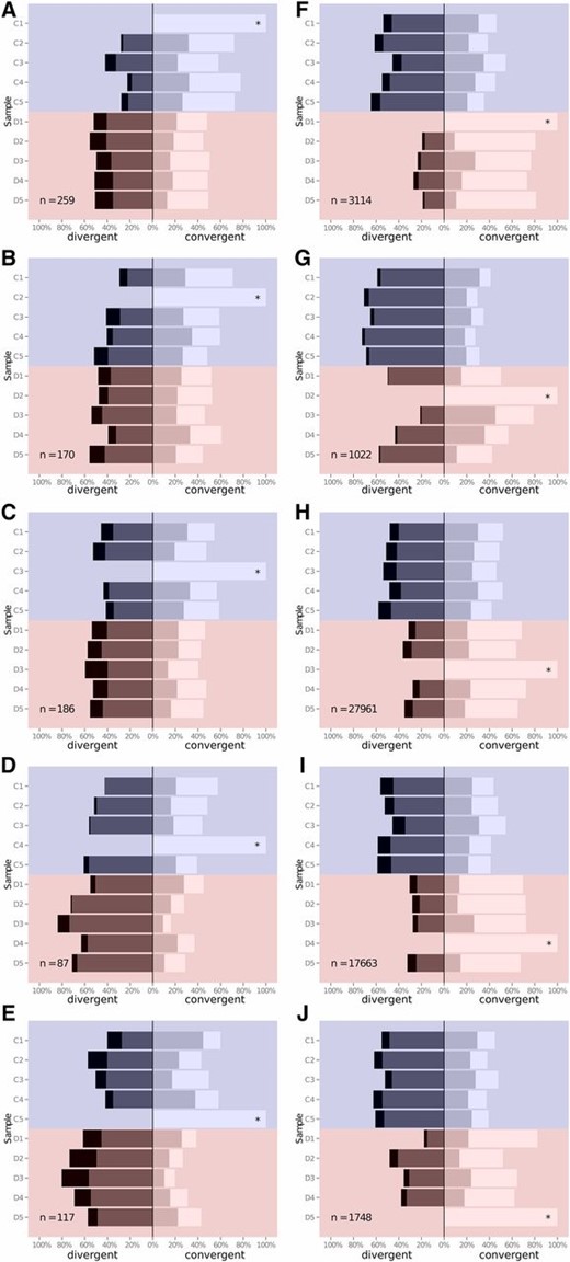
Consistency of allele frequency change. Plots show the distribution of allele frequency changes in all lines, focusing on each replicate control line (A–E) or desiccation-selected line (F–J) in turn. For each focal line (indicated with an asterisk), the frequency of each candidate allele, p, that was significantly differentiated between generation 0 and generation 13 was investigated in all other lines (labeled on the y-axis, controls highlighted in blue, and desiccation-selected lines highlighted in red). The distribution of allele frequencies was then categorized as: p > 0.1 (white); 0 < p < 0.1 (light gray); −0.1 < p < 0 (dark gray); or p < −0.1 (black). Each plot shows the breakdown of distribution in these four categories expressed as a percentage of all SNPs investigated. The number of significantly differentiated SNPs in the focal line is shown in the bottom left-hand corner.
Across all the candidate SNP sets, an ANOVA on the proportion of alleles changing in the same direction as in the focal line revealed significant effects of focal line category (control or desiccation-selected; F1,86 = 7.2, P < 0.01), comparison line category (F1,86 = 5.3, P < 0.05) and the interaction between focal and comparison line category (F1,86 = 94, P < 1 × 10⁻¹⁴).
Gene list overlap
Many of the putative lab-adaptation genes also appeared in the desiccation-replicate gene lists (Figure S13 and File S2), and this overlap was significantly higher than expected for D2, D3, and D4, but not for replicates D1 and D5 (Figure S14). This appears to confirm that laboratory conditions exerted selection pressure on desiccation replicates, as well as controls, even over the relatively short span of this experiment, and justifies the removal of putative lab-adaptation genes from desiccation replicates. Overlap among control-replicate candidate gene lists was higher than expected in all cases (Figure 1M and Figure S15).
After excluding putative lab-adaptation genes, desiccation gene lists often showed no more similarity among replicates than expected by chance (Figure S16 and Figure S17). The exceptions were the overlap among replicates D1, D4, and D5, which showed significantly greater overlap than expected both in pair combinations (Figure 1N and Figure S14, C–D and J), and as a trio (Figure S16, P); 936 genes were shared between D1 and D4 (57.7% of all D1 candidate genes and 21.3% of D4 candidate genes); 240 were shared between D1 and D5 (14.8% of D1 genes and 26.8% of D5 genes); and 409 between D4 and D5 (9.3% of D4 genes and 45.6% of D5 genes); and 195 genes were shared among these three replicates, or 12.0, 4.4, and 21.8% of all D1, D4, and D5 genes respectively. The combinations of D1-D2-D4, D1-D3-D4, D1-D3-D5, D1-D2-D4-D5, and D1-D3-D4-D5 also showed more overlapping genes than expected (Figure S16, L, N, O, W, and X). Most other combinations of replicates did not show significant overlap. We found no evidence that SNPs mapping to multiple genes were driving patterns of gene list overlap (Figure S18 and File S1).
Drift, selection, and effective population size
Effective population size measured at noncandidate SNPs remained moderate despite 21 generations of laboratory culture (Ne = 103–177 across all lines, Figure 3), although it was significantly lower for desiccation replicates (mean Ne = 117) than for controls (mean Ne = 156; two-sided t-test P < 0.001). For the desiccation candidate SNPs, the desiccation replicates all exhibited a drastically lower estimated Ne than did the controls (control mean Ne = 115, desiccation mean Ne = 30, P < 1 × 10⁻⁵) as expected because allelic changes at these SNPs should exceed expectations based on drift. The opposite pattern was observed in the lab-adaptation candidate SNPs, with the desiccation replicates remaining higher than the controls (control mean Ne = 33, desiccation mean Ne = 70, P < 1 × 10⁻⁴). Interestingly, the control replicates exhibited a similar reduction in Ne at the desiccation candidate SNPs to the level of Ne reduction shown by the desiccation replicates at the lab-adapted SNPs (mean reduction in desiccation-selected Ne between neutral and lab-adaptation loci = 41, mean reduction in control Ne between neutral and desiccation candidate loci = 47, P = 0.40). This may indicate the presence in the desiccation replicates of extra lab-adaptation loci that did not reach the significance threshold for allelic differentiation in the control replicates.
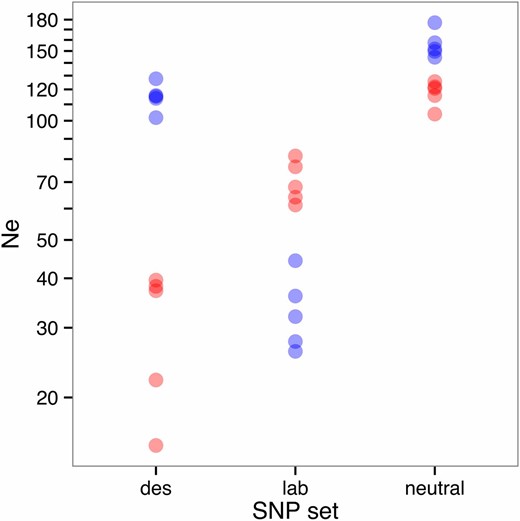
Effective population size for each replicate line, calculated over candidate and noncandidate SNPs. Each point represents the mean effective population size for a desiccation-selected line (red), or control line (blue), calculated over all desiccation candidate SNPs (“des,” n = 38,150–41,624), all lab-adaptation SNPs (“lab,” n = 658–710), or a set of randomly chosen neutral (noncandidate) SNPs (“neutral,” n = 4773–5838). SNP numbers vary slightly among replicates because missing or nonvariable SNPs were excluded.
Mirroring the effective population size results, variance in final allele frequency among replicates increased at loci under selection (Figure 4A). For neutral loci, divergence was low on average (mean f ± SD = 0.09 ± 0.11 among control replicates, 0.12 ± 0.14 among desiccation replicates). At desiccation candidate SNP loci, control replicates remained little diverged (mean f ± SD = 0.08 ± 0.06) but desiccation replicates showed a significantly higher mean divergence (mean f ± SD = 0.29 ± 0.16, P < 1 × 10⁻¹⁵). The opposite pattern was observed at candidate lab-adaption SNPs (control mean f ± SD = 0.31 ± 0.13, desiccation mean f ± SD = 0.11 ± 0.10, P < 1 × 10⁻¹⁵). Thus, both laboratory adaptation and desiccation selection appeared to be driving divergence of replicates rather than convergence. There was a positive relationship between starting allele frequency and variance among replicates (Figure S19), as expected.
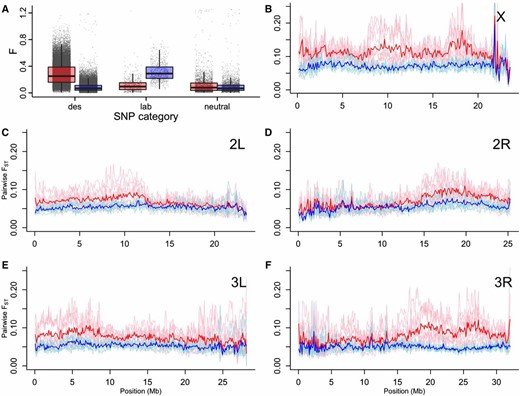
Variance among replicate desiccation lines in allele frequency. (A) Boxplots of standardized variance in allele frequency F (Nicholas and Robertson 1976) among the five desiccation replicates (red) and the five controls (blue) for all desiccation candidate SNPs (“des,” n = 43,242), lab-adaptation candidate SNPs (“lab,” n = 778), and a random subset of SNPs not under selection (“neutral,” n = 4635). Boxplots show the median (thick line), first, and third quartiles (box limits), and values within 1.5× interquartile range from the median (whiskers). The underlying values are shown behind the boxplots. (B–F) Pairwise FST across each chromosome, measured in 100 kbp windows. Pairwise comparisons among desiccation, and among control, replicates are shown in pink and pale blue, respectively; the red line shows the mean pairwise FST across all desiccation replicate pairs; the dark blue line shows the mean pairwise FST across all control replicate pairs.
At the genome-wide scale, mean pairwise FST measured in 100 kbp genomic windows among desiccation replicates was notably higher than among control replicates across the majority of chromosomes X and 3, and for the distal regions of chromosome 2 (Figure 4, B–F).
GO, developmental stage and body part enrichment
Control-line GO category results were dominated by terms associated with mitochondrial activity (File S4); these were “enriched” due to a few SNPs that were located within 1000 bp of numerous mitochondrial genes. No nonmitochondrial categories were significantly enriched in these replicates. Two of the desiccation replicates showed significant enrichment, but the categories were quite different. Replicate D1 was enriched in genes related to catalytic activity, regulation of histone methylation and metallochaperone activity. D3 showed numerous enriched categories, including body morphogenesis, pole plasm RNA localization, translation initiation factor binding, Golgi organization, transmembrane transporter activity, and cell cycle checkpoint categories (File S4).
Enrichment in developmental stage and body tissue categories showed more consistency across desiccation replicates. Candidate gene lists were significantly enriched in genes expressed at high levels in the early embryo (0–8 and 10–12 hr), in late larval stages (mostly at the later time points of third instar larvae), and in adult stages, in more than one replicate (File S4 and Table 1). Interestingly, replicate D3 exhibited enrichment in adult female stages only, while replicates D1 and D5 exhibited enrichment in adult stages of both sexes, and replicate D4 exhibited enrichment in adult male stages only. This was despite equal contribution of male and female flies to each pool. Control replicates occasionally showed enrichment in developmental stage categories, but this was never significant after FDR correction (Table 1).
Gene enrichment in developmental stage categories across the desiccation-selected (D1–D5) and control replicate (C1–C5) candidate genes
| Developmental Stage | D1 | D2 | D3 | D4 | D5 | C1 | C2 | C3 | C4 | C5 | |
|---|---|---|---|---|---|---|---|---|---|---|---|
| Embryo | 0–2 hr | 0.002 | 0.001 | 0.0001 | 0.41 | 0.00001 | 0.17 | 0.76 | 0.15 | 0.23 | 0.22 |
| 2–4 hr | 0.001 | 0.02 | 0.00004 | 0.07 | 0.03 | 0.18 | 0.36 | 0.03 | 0.61 | 0.15 | |
| 4–6 hr | 0.01 | 0.04 | 0.00002 | 0.002 | 0.95 | 0.09 | 0.18 | 0.07 | 0.74 | 0.14 | |
| 6–8 hr | 0.87 | 0.74 | 0.01 | 0.56 | 0.90 | 0.54 | 0.93 | 0.99 | 0.46 | 0.43 | |
| 8–10 hr | 1.00 | 0.44 | 0.11 | 0.66 | 1.00 | 0.12 | 0.37 | 0.65 | 0.42 | 0.05 | |
| 10–12 hr | 0.79 | 0.35 | 0.00001 | 0.02 | 0.92 | 0.18 | 0.89 | 0.99 | 0.87 | 0.89 | |
| 12–14 hr | 1.00 | 1.00 | 0.85 | 0.92 | 1.00 | 0.22 | 0.97 | 0.98 | 0.57 | 0.86 | |
| 14–16 hr | 1.00 | 1.00 | 1.00 | 1.00 | 1.00 | 0.93 | 0.91 | 0.96 | 0.64 | 0.97 | |
| 16–18 hr | 1.00 | 0.99 | 1.00 | 1.00 | 1.00 | 0.85 | 0.87 | 0.75 | 0.65 | 0.93 | |
| 18–20 hr | 1.00 | 1.00 | 1.00 | 1.00 | 1.00 | 0.99 | 0.83 | 0.91 | 0.80 | 1.00 | |
| 20–22 hr | 1.00 | 1.00 | 1.00 | 1.00 | 0.98 | 0.92 | 0.83 | 0.75 | 0.69 | 1.00 | |
| 22–24 hr | 1.00 | 0.99 | 0.76 | 1.00 | 0.99 | 0.72 | 0.81 | 0.59 | 0.67 | 0.99 | |
| Larva | L1 | 0.99 | 0.98 | 0.89 | 1.00 | 0.92 | 0.93 | 0.96 | 0.93 | 0.85 | 1.00 |
| L2 | 0.07 | 0.11 | 0.07 | 0.0001 | 0.14 | 0.55 | 0.37 | 0.00 | 0.69 | 0.67 | |
| L3 12 hr post molt | 0.12 | 0.17 | 0.08 | 0.06 | 0.65 | 0.73 | 0.42 | 0.24 | 0.62 | 0.18 | |
| L3 dark blue gut PS 1–2 | 0.08 | 0.19 | 0.29 | 0.11 | 0.07 | 0.82 | 0.22 | 0.02 | NA | 0.19 | |
| L3 light blue gut PS 3–6 | 0.28 | 0.44 | 0.52 | 0.04 | 0.004 | 0.64 | 0.60 | 0.31 | NA | 0.89 | |
| L3 clear gut PS 7–9 | 0.01 | 0.03 | 0.29 | 0.0001 | 0.004 | 0.87 | 0.54 | 0.30 | 0.44 | 0.21 | |
| Pupa | White pre pupae | 0.03 | 0.06 | 0.39 | 0.05 | 0.31 | 0.97 | 0.07 | 0.38 | 0.72 | 0.09 |
| WPP plus 12 hr | 0.66 | 0.32 | 0.96 | 0.83 | 0.83 | 0.53 | 0.01 | 0.55 | 0.94 | 0.47 | |
| WPP plus 24 hr | 0.69 | 0.98 | 0.99 | 0.57 | 0.91 | 0.39 | 0.53 | 0.41 | 0.99 | 0.22 | |
| WPP plus 2D | 1.00 | 1.00 | 1.00 | 0.87 | 0.72 | 0.77 | 0.91 | 0.87 | 0.27 | 0.77 | |
| WPP plus 3D | 1.00 | 0.26 | 1.00 | 0.92 | 0.96 | 0.51 | 0.57 | 0.68 | 0.18 | 0.96 | |
| WPP plus 4D | 0.96 | 0.90 | 1.00 | 0.98 | 0.99 | 0.89 | 0.86 | 0.06 | 0.96 | 0.92 | |
| Adult | Female eclosion plus 1D | 0.30 | 0.92 | 0.04 | 0.35 | 0.18 | 0.71 | 0.48 | 0.08 | NA | 0.55 |
| Female eclosion plus 5D | 0.03 | 0.13 | 0.002 | 0.42 | 0.04 | 0.11 | 0.76 | 0.39 | 0.01 | 0.27 | |
| Female eclosion plus 30D | 0.36 | 0.46 | 0.01 | 0.73 | 0.01 | 0.26 | 0.94 | 0.38 | 0.01 | 0.60 | |
| Male eclosion plus 1D | 0.02 | 0.75 | 0.04 | 0.0004 | 0.14 | 0.74 | 0.77 | 0.26 | 0.38 | 0.15 | |
| Male eclosion plus 5D | 0.01 | 0.82 | 0.21 | 0.00001 | 0.32 | 0.24 | 0.81 | 0.20 | 0.67 | 0.16 | |
| Male eclosion plus 30D | 0.001 | 0.38 | 0.08 | 0.001 | 0.01 | 0.36 | 0.86 | 0.43 | 0.54 | 0.56 |
Genes were assigned to developmental stage categories based on their relative expression as described in the text. Gene membership of categories presented here was determined with a threshold of 75% maximum expression level. Uncorrected P-values from Gowinda (Kofler and Schlötterer 2012) are shown. P-values <0.05 are italicised, and P-values that remained significant after FDR correction (performed in Gowinda) are shown in bold. “NA” indicates no test was performed because no genes in the candidate list fell in the relevant category.
| Developmental Stage | D1 | D2 | D3 | D4 | D5 | C1 | C2 | C3 | C4 | C5 | |
|---|---|---|---|---|---|---|---|---|---|---|---|
| Embryo | 0–2 hr | 0.002 | 0.001 | 0.0001 | 0.41 | 0.00001 | 0.17 | 0.76 | 0.15 | 0.23 | 0.22 |
| 2–4 hr | 0.001 | 0.02 | 0.00004 | 0.07 | 0.03 | 0.18 | 0.36 | 0.03 | 0.61 | 0.15 | |
| 4–6 hr | 0.01 | 0.04 | 0.00002 | 0.002 | 0.95 | 0.09 | 0.18 | 0.07 | 0.74 | 0.14 | |
| 6–8 hr | 0.87 | 0.74 | 0.01 | 0.56 | 0.90 | 0.54 | 0.93 | 0.99 | 0.46 | 0.43 | |
| 8–10 hr | 1.00 | 0.44 | 0.11 | 0.66 | 1.00 | 0.12 | 0.37 | 0.65 | 0.42 | 0.05 | |
| 10–12 hr | 0.79 | 0.35 | 0.00001 | 0.02 | 0.92 | 0.18 | 0.89 | 0.99 | 0.87 | 0.89 | |
| 12–14 hr | 1.00 | 1.00 | 0.85 | 0.92 | 1.00 | 0.22 | 0.97 | 0.98 | 0.57 | 0.86 | |
| 14–16 hr | 1.00 | 1.00 | 1.00 | 1.00 | 1.00 | 0.93 | 0.91 | 0.96 | 0.64 | 0.97 | |
| 16–18 hr | 1.00 | 0.99 | 1.00 | 1.00 | 1.00 | 0.85 | 0.87 | 0.75 | 0.65 | 0.93 | |
| 18–20 hr | 1.00 | 1.00 | 1.00 | 1.00 | 1.00 | 0.99 | 0.83 | 0.91 | 0.80 | 1.00 | |
| 20–22 hr | 1.00 | 1.00 | 1.00 | 1.00 | 0.98 | 0.92 | 0.83 | 0.75 | 0.69 | 1.00 | |
| 22–24 hr | 1.00 | 0.99 | 0.76 | 1.00 | 0.99 | 0.72 | 0.81 | 0.59 | 0.67 | 0.99 | |
| Larva | L1 | 0.99 | 0.98 | 0.89 | 1.00 | 0.92 | 0.93 | 0.96 | 0.93 | 0.85 | 1.00 |
| L2 | 0.07 | 0.11 | 0.07 | 0.0001 | 0.14 | 0.55 | 0.37 | 0.00 | 0.69 | 0.67 | |
| L3 12 hr post molt | 0.12 | 0.17 | 0.08 | 0.06 | 0.65 | 0.73 | 0.42 | 0.24 | 0.62 | 0.18 | |
| L3 dark blue gut PS 1–2 | 0.08 | 0.19 | 0.29 | 0.11 | 0.07 | 0.82 | 0.22 | 0.02 | NA | 0.19 | |
| L3 light blue gut PS 3–6 | 0.28 | 0.44 | 0.52 | 0.04 | 0.004 | 0.64 | 0.60 | 0.31 | NA | 0.89 | |
| L3 clear gut PS 7–9 | 0.01 | 0.03 | 0.29 | 0.0001 | 0.004 | 0.87 | 0.54 | 0.30 | 0.44 | 0.21 | |
| Pupa | White pre pupae | 0.03 | 0.06 | 0.39 | 0.05 | 0.31 | 0.97 | 0.07 | 0.38 | 0.72 | 0.09 |
| WPP plus 12 hr | 0.66 | 0.32 | 0.96 | 0.83 | 0.83 | 0.53 | 0.01 | 0.55 | 0.94 | 0.47 | |
| WPP plus 24 hr | 0.69 | 0.98 | 0.99 | 0.57 | 0.91 | 0.39 | 0.53 | 0.41 | 0.99 | 0.22 | |
| WPP plus 2D | 1.00 | 1.00 | 1.00 | 0.87 | 0.72 | 0.77 | 0.91 | 0.87 | 0.27 | 0.77 | |
| WPP plus 3D | 1.00 | 0.26 | 1.00 | 0.92 | 0.96 | 0.51 | 0.57 | 0.68 | 0.18 | 0.96 | |
| WPP plus 4D | 0.96 | 0.90 | 1.00 | 0.98 | 0.99 | 0.89 | 0.86 | 0.06 | 0.96 | 0.92 | |
| Adult | Female eclosion plus 1D | 0.30 | 0.92 | 0.04 | 0.35 | 0.18 | 0.71 | 0.48 | 0.08 | NA | 0.55 |
| Female eclosion plus 5D | 0.03 | 0.13 | 0.002 | 0.42 | 0.04 | 0.11 | 0.76 | 0.39 | 0.01 | 0.27 | |
| Female eclosion plus 30D | 0.36 | 0.46 | 0.01 | 0.73 | 0.01 | 0.26 | 0.94 | 0.38 | 0.01 | 0.60 | |
| Male eclosion plus 1D | 0.02 | 0.75 | 0.04 | 0.0004 | 0.14 | 0.74 | 0.77 | 0.26 | 0.38 | 0.15 | |
| Male eclosion plus 5D | 0.01 | 0.82 | 0.21 | 0.00001 | 0.32 | 0.24 | 0.81 | 0.20 | 0.67 | 0.16 | |
| Male eclosion plus 30D | 0.001 | 0.38 | 0.08 | 0.001 | 0.01 | 0.36 | 0.86 | 0.43 | 0.54 | 0.56 |
Genes were assigned to developmental stage categories based on their relative expression as described in the text. Gene membership of categories presented here was determined with a threshold of 75% maximum expression level. Uncorrected P-values from Gowinda (Kofler and Schlötterer 2012) are shown. P-values <0.05 are italicised, and P-values that remained significant after FDR correction (performed in Gowinda) are shown in bold. “NA” indicates no test was performed because no genes in the candidate list fell in the relevant category.
All five desiccation replicates showed significant enrichment of ovary genes (Table 2). Multiple replicates were also enriched in larval tubule and larval fat body genes, with individual replicates further enriched in larval midgut, larval salivary gland, male accessory gland, or testis (after FDR correction).
Gene enrichment in body tissue categories across the desiccation-selected (D1–D5) and control replicate (C1–C5) candidate genes (with SNPs differentiated between the mass-bred and generation 13 pools)
| Body Tissue | D1 | D2 | D3 | D4 | D5 | C1 | C2 | C3 | C4 | C5 |
|---|---|---|---|---|---|---|---|---|---|---|
| Adult carcass | 0.60 | 0.22 | 0.43 | 0.25 | 0.09 | 0.90 | 0.95 | 0.47 | 0.76 | 0.32 |
| Adult fatbody | 0.71 | 0.17 | 0.81 | 0.03 | 0.54 | 0.95 | 0.22 | 0.82 | 0.19 | 0.39 |
| Adult salivary gland | 0.09 | 0.27 | 0.10 | 0.75 | 0.50 | 0.89 | 0.53 | 0.54 | 0.71 | 0.58 |
| Brain | 1.00 | 1.00 | 1.00 | 1.00 | 1.00 | 0.89 | 0.99 | 0.97 | 0.99 | 0.87 |
| Crop | 0.56 | 0.78 | 0.47 | 0.90 | 0.31 | 0.82 | 0.73 | 0.71 | 0.42 | 0.85 |
| Eye | 0.95 | 0.06 | 0.45 | 0.95 | 0.03 | 0.93 | 0.90 | 0.77 | 0.81 | 0.42 |
| Heart | 0.93 | 0.02 | 0.16 | 0.25 | 0.62 | 0.33 | 0.07 | 0.57 | 0.88 | 0.55 |
| Hindgut | 0.69 | 0.72 | 0.32 | 0.64 | 0.77 | 0.23 | 0.54 | 0.28 | 0.53 | 0.92 |
| Larval carcass | 0.98 | 0.80 | 0.94 | 0.99 | 0.91 | 0.38 | 0.79 | 0.09 | 0.72 | 0.87 |
| Larval CNS | 0.75 | 0.35 | 0.59 | 0.93 | 0.39 | 0.25 | 0.78 | 0.85 | 0.42 | 0.68 |
| Larval fatbody | 0.05 | 0.20 | 0.004 | 0.001 | 0.74 | 0.89 | 0.07 | 0.52 | 0.91 | 0.23 |
| Larval hindgut | 0.71 | 0.63 | 0.76 | 0.78 | 0.94 | 0.99 | 0.35 | 0.18 | 0.90 | 0.82 |
| Larval midgut | 0.01 | 0.33 | 0.33 | 0.07 | 0.41 | 0.31 | 0.73 | 0.03 | 0.40 | 0.05 |
| Larval salivary gland | 0.41 | 0.15 | 0.00001 | 0.42 | 0.53 | 0.17 | 0.68 | 0.16 | 0.82 | 0.15 |
| Larval trachea | 0.82 | 0.73 | 0.96 | 0.72 | 0.93 | 0.21 | 0.49 | 0.94 | 0.77 | 0.82 |
| Larval tubule | 0.02 | 0.0001 | 0.27 | 0.18 | 0.16 | 0.39 | 0.41 | 0.70 | 0.54 | 0.10 |
| Male accessory gland | 0.07 | 0.15 | 0.00001 | 0.33 | 0.08 | 0.25 | 0.56 | 0.91 | 0.06 | 0.35 |
| Midgut | 0.21 | 0.87 | 0.75 | 0.17 | 0.14 | 0.09 | 0.20 | 0.02 | 0.18 | 0.04 |
| Ovary | 0.00001 | 0.02 | 0.00001 | 0.02 | 0.0001 | 0.25 | 0.49 | 0.63 | 0.03 | 0.02 |
| Spermatheca virgin | 0.29 | 0.61 | 0.06 | 0.01 | 0.67 | 0.52 | 0.61 | 0.56 | 0.71 | 0.86 |
| Testis | 0.09 | 0.27 | 0.26 | 0.00001 | 0.55 | 0.46 | 0.34 | 0.12 | 0.64 | 0.30 |
| Thoracicoabdominal ganglion | 0.93 | 0.85 | 0.98 | 0.99 | 0.97 | 0.95 | 0.63 | 1.00 | 0.90 | 0.68 |
| Tubule | 0.02 | 0.28 | 0.12 | 0.16 | 0.71 | 0.48 | 0.37 | 0.07 | 0.29 | 0.73 |
Genes were assigned to tissue categories based on their relative expression as described in the text. Gene membership of categories presented here was determined with a threshold of 75% maximum expression level. Uncorrected P-values from Gowinda (Kofler and Schlötterer 2012) are shown. P-values <0.05 are italicised, and P-values that remained significant after FDR correction (in Gowinda) are shown in bold.
| Body Tissue | D1 | D2 | D3 | D4 | D5 | C1 | C2 | C3 | C4 | C5 |
|---|---|---|---|---|---|---|---|---|---|---|
| Adult carcass | 0.60 | 0.22 | 0.43 | 0.25 | 0.09 | 0.90 | 0.95 | 0.47 | 0.76 | 0.32 |
| Adult fatbody | 0.71 | 0.17 | 0.81 | 0.03 | 0.54 | 0.95 | 0.22 | 0.82 | 0.19 | 0.39 |
| Adult salivary gland | 0.09 | 0.27 | 0.10 | 0.75 | 0.50 | 0.89 | 0.53 | 0.54 | 0.71 | 0.58 |
| Brain | 1.00 | 1.00 | 1.00 | 1.00 | 1.00 | 0.89 | 0.99 | 0.97 | 0.99 | 0.87 |
| Crop | 0.56 | 0.78 | 0.47 | 0.90 | 0.31 | 0.82 | 0.73 | 0.71 | 0.42 | 0.85 |
| Eye | 0.95 | 0.06 | 0.45 | 0.95 | 0.03 | 0.93 | 0.90 | 0.77 | 0.81 | 0.42 |
| Heart | 0.93 | 0.02 | 0.16 | 0.25 | 0.62 | 0.33 | 0.07 | 0.57 | 0.88 | 0.55 |
| Hindgut | 0.69 | 0.72 | 0.32 | 0.64 | 0.77 | 0.23 | 0.54 | 0.28 | 0.53 | 0.92 |
| Larval carcass | 0.98 | 0.80 | 0.94 | 0.99 | 0.91 | 0.38 | 0.79 | 0.09 | 0.72 | 0.87 |
| Larval CNS | 0.75 | 0.35 | 0.59 | 0.93 | 0.39 | 0.25 | 0.78 | 0.85 | 0.42 | 0.68 |
| Larval fatbody | 0.05 | 0.20 | 0.004 | 0.001 | 0.74 | 0.89 | 0.07 | 0.52 | 0.91 | 0.23 |
| Larval hindgut | 0.71 | 0.63 | 0.76 | 0.78 | 0.94 | 0.99 | 0.35 | 0.18 | 0.90 | 0.82 |
| Larval midgut | 0.01 | 0.33 | 0.33 | 0.07 | 0.41 | 0.31 | 0.73 | 0.03 | 0.40 | 0.05 |
| Larval salivary gland | 0.41 | 0.15 | 0.00001 | 0.42 | 0.53 | 0.17 | 0.68 | 0.16 | 0.82 | 0.15 |
| Larval trachea | 0.82 | 0.73 | 0.96 | 0.72 | 0.93 | 0.21 | 0.49 | 0.94 | 0.77 | 0.82 |
| Larval tubule | 0.02 | 0.0001 | 0.27 | 0.18 | 0.16 | 0.39 | 0.41 | 0.70 | 0.54 | 0.10 |
| Male accessory gland | 0.07 | 0.15 | 0.00001 | 0.33 | 0.08 | 0.25 | 0.56 | 0.91 | 0.06 | 0.35 |
| Midgut | 0.21 | 0.87 | 0.75 | 0.17 | 0.14 | 0.09 | 0.20 | 0.02 | 0.18 | 0.04 |
| Ovary | 0.00001 | 0.02 | 0.00001 | 0.02 | 0.0001 | 0.25 | 0.49 | 0.63 | 0.03 | 0.02 |
| Spermatheca virgin | 0.29 | 0.61 | 0.06 | 0.01 | 0.67 | 0.52 | 0.61 | 0.56 | 0.71 | 0.86 |
| Testis | 0.09 | 0.27 | 0.26 | 0.00001 | 0.55 | 0.46 | 0.34 | 0.12 | 0.64 | 0.30 |
| Thoracicoabdominal ganglion | 0.93 | 0.85 | 0.98 | 0.99 | 0.97 | 0.95 | 0.63 | 1.00 | 0.90 | 0.68 |
| Tubule | 0.02 | 0.28 | 0.12 | 0.16 | 0.71 | 0.48 | 0.37 | 0.07 | 0.29 | 0.73 |
Genes were assigned to tissue categories based on their relative expression as described in the text. Gene membership of categories presented here was determined with a threshold of 75% maximum expression level. Uncorrected P-values from Gowinda (Kofler and Schlötterer 2012) are shown. P-values <0.05 are italicised, and P-values that remained significant after FDR correction (in Gowinda) are shown in bold.
Protein–protein interaction networks
In four out of five desiccation replicates, more of the candidate genes formed a protein–protein interaction network than expected (Figure S20, A–E). For all five replicates, the number of connections in the resulting network was also higher than expected (Figure S20, F–J). We investigated two possible explanations for this: first, that more of the genes in our candidate lists were annotated with known interactions than expected by chance; second, that our candidate gene lists formed better-connected networks than expected by chance. We found that the first possibility was the case (Figure S20, K–O); more of our candidate genes had known interactions than did the simulated gene selection, on average, and this was significant in three replicates. In fact, by simulating random subnetworks of the same size as our real networks, it was clear that the real networks actually had lower density (lower average connections per node) than expected by chance (Figure S20, P–T).
A null distribution for overlap among each pair and trio of network replicates was built by calculating overlap among zero-degree networks made from the gene lists obtained by SNP resampling (maintaining LD). When compared against the SNP-level permutation expectation, observed overlap was not significantly different from that expected for network pairs, whether measured as node overlap (Figure S21, A–J) or edge overlap (Figure S21, K–T), except for the pairs of D1 and D4, D1 and D5, and D2 and D3 (Figure S21, C–E and M–O), where overlap was higher than expected. Overlap among trios of networks was within expected levels in every case (Figure S21, U–AN) except the combination of D1, D4, and D5, where again overlap was higher (Figure S21, Z and AJ).
Discussion
In this study, we assessed the genetic changes across a set of replicated selection lines. We initiated the base population at a reasonable size to reduce LD, ensuring that a substantial number of flies were turned over during the selection process every generation, and maintained an equal number of replicate control lines to improve our ability to assess the repeatability of selection responses. Under truncating selection, we expected to have adequate power to detect changes in many QTL of large effect size (Kessner and Novembre 2015). Moreover, our effective population size (Ne) remained moderate across neutral markers for all replicate lines (Figure 3), indicating that we avoided effects of substantial genetic drift. We also maintained separate independent control lines to allow laboratory adaptation to be separated from selection effects, and used the results to understand the genetic architecture underlying replicate selection responses. Despite these precautions, we had limited success in identifying consistent genetic changes across the replicate lines. Instead, we observed large differences in the number of loci estimated as contributing to the selection response, likely reflecting hitchhiking effects and different selection responses in the replicate lines.
Genetic changes underlying laboratory adaptation
As expected given the short time the base population had been in the laboratory, we found evidence of laboratory adaptation as reflected by genetic changes in the control lines compared to the base population. We interpreted any gene present in at least one control-replicate candidate gene list as a putative lab-adaptation gene, giving a total of 702 such genes. These genes were significantly enriched in three of the five desiccation replicates as well (Figure S14), which were also expected to undergo laboratory adaptation. The line differences in genetic changes underlying laboratory adaptation is consistent with phenotypic observations suggesting that lines can, to some extent, develop their own trajectories of laboratory adaptation, although consistent phenotypic changes also occur (Griffiths et al. 2005; Santos et al. 2012). We then took a conservative approach toward separating the effects of laboratory adaptation from desiccation selection by removing all putative lab-adaptation genes from desiccation candidate gene lists for further analysis.
Many of the changes were common to the different control lines; at the gene level, all control replicates shared more genes than expected by chance, except for the combination of replicates C3 and C4 (Figure 1L and Figure S15). This was largely driven by mitochondrial SNPs, which typically mapped to multiple genes. The four candidate genes found in all control replicate lists were located within a 2600-bp mitochondrial region: ND4, ND4L, ND5, and tRNA:H. Mitochondrial genes also dominated the GO ontology enrichment results for the control replicates, producing enrichment in mitochondrial, respiration, and oxidoreductase activity categories significant across all lines except C4 (File S4). The functional significance of these SNP frequency changes are not known, and are difficult to interpret since the mitochondrial genome is inherited as a single, fully linked locus, but they may influence metabolism, as naturally occurring mitochondrial DNA variants have been shown previously to confer variation in metabolic function in Drosophila (Pichaud et al. 2012).
Genetic changes underlying desiccation resistance
The proportion of the genome responding to desiccation selection differed greatly among replicates, with lines D3 and D4 showing ∼10× as many candidate SNPs as the other three replicates (Figure 1 and Table S1). There were indications of a possible relationship between sequencing coverage depth and candidate SNP number (Table S1), despite stringent and consistent multiple-testing corrections. Determining the statistically optimum correction approach for a PoolSeq experiment is an important methodological research question as yet unanswered (Lynch et al. 2014).
At the chromosome scale, large disparate genomic regions appeared to be responding to selection (Figure 1 and Figure S2). A likely explanation for this pattern is that low-frequency, large-effect alleles under selection caused extensive genetic hitchhiking early in the experiment in some replicates, while being lost from other replicates due to stochastic recruitment from the starting population or genetic drift. We identified some inconsistent evidence for enrichment of low-starting-frequency alleles in highly differentiated chromosomal windows (Figure S2 and Figure S6). We performed a power analysis that predicted a low rate of long-distance LD (Table S2). However, it still seems likely that low-frequency alleles contributed to the divergence among replicate lines, and contributed to long-distance LD across haplotype blocks. Similar patterns of apparent haplotype blocks have been observed in other E&R studies (Burke et al. 2010; Turner et al. 2011; Orozco-terWengel et al. 2012; Turner and Miller 2012), even those that identified candidate loci as those showing a common signal between replicates. A “block-like” pattern is also evident in Manhattan plots generated in a simulation study (Kofler and Schlötterer 2013). In this study, with 150 true positive SNPs, only the “high-budget” design (10 replicates, 2000 individuals each, 120 generations), run with a high selection coefficient per marker, produced clear peaks as opposed to blocks. Our “low-budget” design was likely still underpowered, especially if the genetic basis of desiccation resistance can indeed involve a very large number of small-effect loci. However, further data are required to identify the exact mechanism by which haplotype blocks seem to respond to selection, ideally from resequenced individual fly haplotypes (Franssen et al. 2014).
Despite this issue, the results do point to numerous candidate genomic regions contributing to the selection response, consistent with the fact that desiccation resistance is a complex trait with a number of underlying physiological and morphological traits potentially contributing to resistance (Hoffmann and Parsons 1989b; Hoffmann and Harshman 1999; Gibbs et al. 2003; Chown et al. 2011; Rajpurohit et al. 2013). In agreement, a previous selection study using microarray hybridization (Telonis-Scott et al. 2012), and a Pool-GWAS study (Telonis-Scott et al. 2016), found numerous genomic regions associated with desiccation resistance.
Candidate SNP sets for both laboratory adaptation (4/5 replicates), and for desiccation-resistance (5/5 replicates), were significantly enriched in exonic SNPs and showed underenrichment of intergenic SNPs (Figure S9). A few candidate SNPs were predicted to have a high impact on protein function, by disrupting either a stop codon or a splice site, but only one of these was found in multiple desiccation replicates. This mitochondrial SNP was predicted to cause a stop codon loss in the ND5 gene, which encodes a member of the NADH dehydrogenase complex I, part of the respiratory chain. This SNP may impact metabolic rate; indeed, reduced metabolic rate is one intermediate phenotype previously linked to desiccation resistance (Hoffmann and Harshman 1999). The other putative high-impact SNPs were located in high-level regulatory genes (e.g., tim, bowl, Pez, and REPTOR), signaling-pathway genes involved in tissue organization (csw, cv-d, and spn-B), and genes with more specific functions including muscle contraction (Tm1), ion channel components (Shaw), eggshell membrane structure (Vm32E), cell adhesion (Dscam3), known (Ir47a, Or33b), and putative (Gr98c) taste or odorant receptors, fatty acid oxidation (CRAT), terminal N-linked glycan synthesis (GalT1), along with numerous other genes with little-understood or completely unknown function (Table S4). All desiccation replicates were also significantly enriched in 5′-UTR SNPs. SNP locations previously identified as eQTLs/veQTLs (Huang et al. 2015) were significantly overrepresented in all desiccation replicates (Figure S11). Together, these results point to the likely involvement of gene expression regulation in the desiccation resistance phenotype, as previously suggested (Matzkin and Markow 2009; Sinclair et al. 2013), and which may explain why this trait appears controlled by many small-effect loci (Ayala and McDonald 1980).
Significant overlap among some candidate desiccation SNP sets indicates that replicate lines have harnessed different but partly overlapping suites of loci to adapt to desiccation stress. Many were intergenic, which explains the somewhat different results observed for gene-level overlap. Overlap at the level of genes targeted by the putative eQTL candidate SNPs, was not significantly higher than expected for any combination of desiccation replicates (Figure S12). At the functional level, GO category enrichment analysis did not indicate noticeable overlap, with only replicates D1 and D3 showing significantly enriched categories, which did not overlap. The list of 13 genes identified as candidates in all five desiccation replicates was dominated by very long (>20 kbp) genes or regions, and hence likely includes false positive hits (see File S1 and Figure S22 for further details). Cdk1 remains an intriguing candidate: it is relatively short (1523 bp), and yet appeared as a candidate gene in all five replicate lines. This gene encodes cyclin-dependent kinase 1, a crucial protein kinase controlling mitotic cell cycle stage transitions by phosphorylating numerous cellular proteins.
Functional and network-level overlap among desiccation replicates
When we instead classified genes according their known expression level in body part or developmental stage categories, we found significant enrichment in all desiccation replicates for genes expressed at a high level in the ovary (Table 2), and in early embryo stages (Table 1), with 4/5 replicates enriched in genes expressed in midlarval stages, 3/5 replicates enriched in adult female stages, and 3/5 enriched in adult male stages (Table 1). Two out of five replicates were also enriched in larval fat body-expressed genes, and a different two enriched in larval tubule-expressed genes (Table 2). Although it is difficult to pinpoint a specific link between ovary gene expression and desiccation resistance, this result is in line with previous reports of enrichment of reproduction-related genes in desiccation-stressed Drosophila mojavensis (Rajpurohit et al. 2013). It may implicate maternal effects in this trait, and may provide some support to previous suggestions that early developmental stages can be important in energy/body weight accumulation that contributes to adult desiccation resistance (Chippindale et al. 1998).
As well as showing significant candidate gene overlap, replicate pairs D1–D4 and D1–D5 shared more edges than expected by chance in zero-order protein–protein interaction networks, which persisted at the D1–D4–D5 trio level. All desiccation-replicate networks were larger than expected, which appeared due to an overrepresentation of genes with any known interactions (as opposed to an overrepresentation of genes with high connectivity). This may indicate the desiccation candidate genes tend to be pleiotropic—that they are involved in numerous phenotypic traits, and so tend to have been investigated previously with respect to function—or that they tend to be involved in protein–protein interactions rather than in DNA–protein or other molecular interactions within the cell.
Convergence/divergence under selection
Whether adaptation to the same selective pressure should cause distinct populations to diverge or converge is a question of longstanding interest in evolutionary biology (Cohan and Hoffmann 1989; Arendt and Reznick 2008). Prior to the advent of genome sequencing, quantitative genetic experiments attempted to indirectly identify whether evolution proceeded in parallel or using different genes. These revealed evidence for multiple genetic trajectories for D. melanogaster ethanol tolerance (Cohan and Hoffmann 1986), and possibly for D. serrata desiccation resistance (Cohan and Hoffmann 1989; Blows and Hoffmann 1993), as well as Drosophila learning ability (Kawecki and Mery 2006) and maternal effects on larval nutrition state (Vijendravarma and Kawecki 2015). Here, we show that loci capable of responding to selection exhibit apparently strong divergence across replicate populations compared to neutral loci, and that the resulting mean divergence extends across large regions of the genome (Figure 4). This is likely due to SNPs in candidate regions showing substantial frequency change differences in different lines that increase the mean FST even over relatively large genomic windows. Thus, while there is evidence of drift among replicate lines at neutral loci consistent with previous results (Simões et al. 2008, 2010), this points to selection increasing divergence at the genomic level, as the variance in allele frequencies is relatively higher for loci in genomic regions under selection than for neutral loci.
Evolutionary repeatability
Closely tied to the question of “divergence vs. convergence” is the issue of evolutionary repeatability. At the genomic level, many examples of parallel phenotypic evolution implicate some repeatable, and some distinct, loci (Bradic et al. 2013; Elmer et al. 2014; Bailey et al. 2015). For example, the threespine stickleback (Gasterosteus aculeatus) has repeatedly lost plate armor during freshwater colonization. The molecular mechanism underlying this parallel evolution involves a combination of homologous and independently evolved alleles (Colosimo et al. 2005; Chan et al. 2010; Deagle et al. 2012; Jones et al. 2012). The extent to which evolution is repeatable is expected to depend on the genetic basis of a trait, and how far adaptation has already progressed. A phenotypic trait with a complex genetic basis is by definition predicted to exhibit lower evolutionary repeatability than a simple trait. Under the mutational landscape model, the probability of parallel evolution is 2/(n+1) where n = the number of beneficial mutations the species has available (Orr 2005). Thus the probability of parallel evolution is dependent on genome size (Orr 2005). As adaptation proceeds, and a fitness peak is approached, repeatability should increase (Bailey et al. 2015) because fewer pathways are available; but, when multiple fitness peaks exist, repeatability may always remain low.
Given that desiccation resistance showed a polygenic genetic basis, the mutational landscape model predicts little parallel evolution across the replicate lines. This approach may have underestimated candidate SNP overlap due to coverage depth variation among replicates, and stringent coverage depth requirements for SNPs to be detected as significantly differentiated. It also had limited power to detect true differentiated SNPs (true positive rate: 0.4), which implies that many cases of overlap were missed. However, although the candidate SNP sets largely differed across replicates, they did overlap significantly, both among the control replicates (Figure S7) and among the desiccation replicates (Figure S8), indicating some convergence. The direction of allele frequency change was also quite consistent among replicates within each selection regime (Figure 2), suggesting that, while significant changes in alleles may have tended to differ among the replicate lines, there was still a tendency for selection to push alleles in the same direction. Assuming that selection can be continued for a long period in large populations, there is then a question of whether replicate lines might start to converge for alleles under continuous directional selection, particularly as LD is broken down through ongoing recombination.
The question of how best to identify heterogeneous genomic trajectories to the same phenotype is still open. When the detection of significantly changing alleles relies on their presence in multiple replicate lines (e.g., Orozco-terWengel et al. 2012), or multiple natural populations, for that matter (Bradic et al. 2013; Roesti et al. 2014), it is not possible to test whether trajectories are independent. The most high-powered experimental evolution study to date still failed to robustly identify replicate-specific loci contributing to a phenotype (Burke et al. 2014). In our lines, we can therefore only conclude that the repeatability of selection response under desiccation appears low although it is still detectable. Whether it would have become more apparent with additional steps to decrease hitchhiking effects, and/or additional generations of selection remains unclear.
Concluding remarks
Results from the current set of experiments meet expectations based on quantitative genetic theory, but also reflect the limitations of selection experiments to detect specific loci under selection. For a classic physiological trait with a clear connection to the ecology of Drosophila species, and multiple options for selection responses, there is a polygenic response to desiccation selection that differs between replicate lines, even though selected alleles are being pushed in the same direction. Differences in the genomic basis of resistance between lines may partly reflect hitchhiking effects but also indicates that the same selection pressures imposed on species at an effective population size of around 100 can lead to diverse outcomes that are evident at the SNP, gene and higher levels. The trait selected has a high heritability in D. melanogaster (Hoffmann and Parsons 1989b, 1993; Kellermann et al. 2009), and selection can produce lines with a very high level of resistance (Chippindale et al. 1998) as a consequence of rapid changes that can be obtained when population sizes are substantial. These patterns are consistent with the notion that multiple genetic changes underlie the selection response. However, desiccation selection has also been associated with consistent costs across lines, suggesting common mechanistic responses (Hoffmann and Parsons 1989b; Chippindale et al. 1998).
Understanding the repeatability of evolution is a major goal of evolutionary biology. Even now, in the age of evolutionary genomics, most studies focus on common patterns across experimental replicates, and do not attempt to tackle differences among them because the analytical framework to do so is lacking or requires power in excess of what is generally available (Burke et al. 2014). The risk is that, by focusing on convergent patterns and avoiding consideration of replicate line differences, we may be ignoring a large swathe of genomic variation that has the capacity to contribute to phenotypic traits. Our finding that selection promotes replicate line divergence is a foreboding result, when we consider that many species currently exist in fragmented populations: if low gene flow coincides with several generations of strong selection pressure (for example, by new climate conditions) that leads to differentiation among populations, Bateson-Dobzhansky-Muller incompatibilities (reviewed in Orr 1996) may reduce subsequent gene flow, and lead to permanent population differentiation. This, in turn, will leave isolated populations at heighted risk of extinction due to small effective population size (Willi and Hoffmann 2009; Bijlsma and Loeschcke 2011): despite adapting to an initial stress, their long-term resilience may be greatly reduced.
Acknowledgments
We would like to thank Charles Robin, Chuck Langley, and John Oakeshott for discussions, and Melissa Davis for advice on network building. We thank the two anonymous reviewers, and, particularly, David Begun, who provided useful and constructive comments that improved the manuscript. We also thank Ronald Lee for collecting the flies, and Lea Rako, Jennifer Shirriffs, Kelly Richardson, Anjali Goundar, and Yoshinori Endo for support with rearing of the laboratory lines. We would also like to thank the Victorian Life Science Computation Initiative (VLSCI) for high-performance computing services. This work was supported by an Australian Research Council (ARC) Laureate Fellowship, and a Science and Industry Endowment Fund grant to A.A.H., and Swiss National Science Foundation grants (PBEZP3_140043 and PA00P3_145372) to S.B.H. The funders had no role in study design, data collection and analysis, decision to publish, or preparation of the manuscript.
Footnotes
Supplemental material is available online at www.genetics.org/lookup/suppl/doi:10.1534/genetics.116.187104/-/DC1.
Communicating editor: D. J. Begun
Literature Cited
Broad Institute, 2014 Picard v1.96. Available at: https://broadinstitute.github.io/picard/
Csardi, G., and T. Nepusz, 2006 The igraph software package for complex network research. InterJournal Complex Systems 1695: 2006. v1.0.1. Available at: http://igraph.org.
Griffin P. C., 2016a griffinp/Sel_Line v0.1: data processing code for ‘genomic trajectories to desiccation resistance’. Available at: https://zenodo.org/record/166394.
Griffin, P. C., 2016b griffinp/desiccation-selection v0.1: code for ‘genomic trajectories to desiccation resistance’. Available at: https://zenodo.org/record/166392.
Pope, B., C. Sloggett, G. Philip, and M. Wakefield, 2013 Rubra: a bioinformatics pipeline. Available at: https://github.com/bjpop/rubra, commit 9b52bd081c.
R Core Team, 2014 R: a language and environment for statistical computing v3.1.0. The R Foundation for Statistical Computing, Vienna, Austria. Available online at http://www.R-project.org/.
Smit A. F. A., R. Hubley, and P. Green, 2013–2015 RepeatMasker Open-4.0.3. Available at: http://www.repeatmasker.org.
