


Abstract
Estimation of epidemiological and population parameters from molecular sequence data has become central to the understanding of infectious disease dynamics. Various models have been proposed to infer details of the dynamics that describe epidemic progression. These include inference approaches derived from Kingman’s coalescent theory. Here, we use recently described coalescent theory for epidemic dynamics to develop stochastic and deterministic coalescent susceptible–infected–removed (SIR) tree priors. We implement these in a Bayesian phylogenetic inference framework to permit joint estimation of SIR epidemic parameters and the sample genealogy. We assess the performance of the two coalescent models and also juxtapose results obtained with a recently published birth–death-sampling model for epidemic inference. Comparisons are made by analyzing sets of genealogies simulated under precisely known epidemiological parameters. Additionally, we analyze influenza A (H1N1) sequence data sampled in the Canterbury region of New Zealand and HIV-1 sequence data obtained from known United Kingdom infection clusters. We show that both coalescent SIR models are effective at estimating epidemiological parameters from data with large fundamental reproductive number and large population size . Furthermore, we find that the stochastic variant generally outperforms its deterministic counterpart in terms of error, bias, and highest posterior density coverage, particularly for smaller and . However, each of these inference models is shown to have undesirable properties in certain circumstances, especially for epidemic outbreaks with close to one or with small effective susceptible populations.
Phylodynamics and the Coalescent
THE epidemiological and evolutionary processes that underpin rapidly evolving species occur on a shared spatiotemporal frame of reference. Unified analyses that include both the dynamics of an epidemic and the reconstruction of the pathogen phylogeny can therefore uncover otherwise inaccessible information to aid in outbreak prevention. Such information includes the rates of pathogen transmission and host recovery, effective population sizes, and the “time of origin” representing the introduction of the first infected individual into a population of susceptible hosts.
The term phylodynamics was popularized by Grenfell et al. (2004) to describe the interlaced study of immunodynamics, epidemiology, and evolutionary mechanisms. Several phylodynamic models, both stochastic and deterministic in nature, have since been developed to characterize the phylogenetic history of the pathogen species and compartmentalizations of the host population throughout the epidemic. Such models grant the ability to infer key epidemiological parameters from genetic sequence data and include birth–death branching processes (Stadler et al. 2012, 2013; Gavryushkina et al. 2014; Kühnert et al. 2014), as well as coalescent approaches (Griffiths and Tavaré 1994; Pybus et al. 2001; Rasmussen et al. 2011, 2014; Koelle and Rasmussen 2012; Dearlove and Wilson 2013) derived from Kingman’s coalescent theory (Kingman 1982).
Significant steps toward the unification of epidemiology and statistical phylogenetics were made by Pybus et al. (2001), Volz et al. (2009), and Dearlove and Wilson (2013), with the formalization and application of Kingman’s n-coalescent to pathogen population dynamics. These methods involved numerical integration of a set of ordinary differential equations (ODEs) to find deterministic approximations to the variation in the number of sampled lineages through time. Volz (2012) extended the tree density calculation from previous work (Volz et al. 2009) to allow for serially sampled and spatially structured genetic sequence data. In this coalescent model, the birth and death rates can vary in time and by the state of the host, so that “the birth rate of a single gene copy is both time- and state-dependent” (Volz 2012, p. 7).
In this article, we assess the ability of coalescent-based phylodynamic models to infer, in a Bayesian setting, a range of epidemiological parameters from simulated data. While Dearlove and Wilson (2013) paved the way by implementing a coalescent approach for deterministic susceptible–infected (SI), susceptible–infected–susceptible (SIS), and susceptible–infected–removed (SIR) models for Bayesian inference, we implement and rigorously test both deterministic and stochastic coalescent SIR models of epidemic dynamics extended for heterochronously sampled data.
Stochastic and Deterministic Models
Stochasticity and determinism in population sizes each maintain dominant roles in particular stages of an epidemic. Once the infected population has grown considerably large, on the order of 1000–10,000 lineages, the probability densities of stochastically expressed population size dynamics converge toward the deterministic interpretation (Rouzine et al. 2001). However, during the early stages the population size of infected individuals is small, and the dynamics of the epidemic are therefore governed by stochastic processes due to the relative significance of fluctuations in the demographic and rate parameters of the population model (Kühnert et al. 2014). Therefore, approximating the prevalence of infection by a deterministic function requires the number of infected hosts within the effective population to be assumed as very large throughout the duration of the described epidemic, i.e., once the exponential growth phase has been reached (Rouzine et al. 2001).
Population size is critical to the epidemiological system and, as with any parameter in a Bayesian setting, yields the most accurate estimations when detailed prior information is available and incorporated into the inference (Drummond et al. 2006). In our extension and implementation of the coalescent model for epidemics, both stochastic and deterministic population size processes are used for the simulation of trees and/or trajectories for subsequent inference.
Compartmental Population Models (SIR)
Host populations can be compartmentalized simply but effectively in mathematical models that describe epidemic progression. The specific division of the aggregate population depends on the contagion, spanning a range of scenarios where hosts may or may not recover from infection, may or may not be reinfected, etc. Such examples include the SI, SIS, and SIR models (Anderson and May 1991; Keeling and Rohani 2008). Each of these compartments can be expressed either (a) by a set of ODEs that describe the deterministic time development of real-valued compartment occupancies or (b) in terms of integer-valued occupancies governed by continuous-time Markov chains (CTMC) that allow for a degree of uncertainty in the timing and number of events that occur over the course of the epidemic.
Both types of epidemic trajectories can be related to models of sampled transmission tree genealogies. In the deterministic case, this relationship is made via the coalescent distributions described in Volz (2012). We call this the deterministic coalescent SIR model. In the stochastic case, genealogies appear naturally from a branching process in which the branching events coincide with the transmission events in the CTMC and only those lineages ancestral to sampled removals are recorded. We call this the stochastic SIR model.
Another way of relating the stochastic SIR model to sampled transmission trees involves drawing a realization of a stochastic SIR epidemic and then using the coalescent distribution in Volz (2012) to produce a tree conditional on the particular piecewise constant infected compartment size corresponding to that realization. We call this approach the stochastic coalescent SIR model. Unlike BDSIR, the stochastic coalescent SIR model does not require the sampling process to be specified explicitly.
Both the transmission rate β and the removal rate γ can be estimated using each of the methods considered in this article from data ascribed to an SIR epidemic.
Methods
Inference framework
Here, , , and represent the host compartment sizes from the present time back to the origin , such that , , and .
The various terms making up the right-hand side of Equation 6 are the tree likelihood , the tree prior , the epidemic trajectory density , and the substitution and epidemiological parameter priors and . The probability is merely a normalizing constant and can be ignored. It is the product of the tree prior and trajectory density that distinguishes each of the models considered in this article.
In contrast, the stochastic coalescent SIR model assumes that the epidemic is generated by a jump process corresponding to the master equation given in Equation 5. In this case, the probability is nonsingular and thus contributes to the uncertainty in the final inference result.
In the BDSIR model introduced by Kuhnert et al. (2014), is the same as for the stochastic coalescent SIR model, but is defined differently. See Kühnert et al. (2014) for details.
Markov chain Monte Carlo algorithm
We use Markov chain Monte Carlo (MCMC) to sample from the joint posterior density given in Equation 6. Many of the specifics of the algorithm used have been discussed previously, in particular the method for calculating the tree likelihood (Felsenstein 1981, 2004) and the mechanism for exploring tree space (Drummond et al. 2002). However, the model-specific product requires special attention.
In the case of the deterministic coalescent SIR model, this density reduces to , meaning that the density of the tree given epidemiological parameters η is obtained simply by substituting the numerical solution to Equations 1–3 for those parameters into Equation 7.
Implementation and validation
We have implemented the schemes described above for performing inference under the deterministic and stochastic coalescent SIR models within the BEAST 2 phylodynamics package found at http://github.com/CompEvol/phylodynamics. This has a number of advantages over a stand-alone implementation. Foremost, we were able to avoid reimplementing components of the algorithm that are in common with other already-implemented phylogenetic and phylodynamic analyses, such as the MCMC proposal operators used to traverse the parameter space. Furthermore, this greatly increases the usefulness of the implementation, as it can be immediately used in conjunction with a wide variety of nucleotide and amino acid substitution models and parameter priors.
We have taken two steps to ensure our implementation is correct. First, we compared tree probability density values calculated using the main implementation of each of the two models with those calculated using completely independent implementations in R (R Core Team 2014).
Second, we used the implemented MCMC algorithms to sample transmission trees from the tree density given in Equation 11 for each model. We then compared the distributions of tree height, total edge length, and binary clade count summary statistics from these sampled ensembles with sample distributions obtained directly via stochastic simulation. As shown in Supporting Information, File S1, Figure S1, Figure S2, and Figure S3 (Sampling from the prior) and in the associated figures, the resulting pairs of distributions agree, providing strong support for our claim that the implementations of the methods described above are correct.
Instructions for downloading and using this package are also available on the project website located at http://github.com/CompEvol/phylodynamics.
Simulation study
To evaluate the implementation and extension of the coalescent models, we performed analyses on both sequence data and fixed trees simulated with known parameter values. The median estimated values produced by each model were then used to measure relative error and bias, along with the widths and coverage of 95% highest posterior density (HPD) intervals.
Stochastic SIR trees and trajectories were generated using master equations in the simulation package MASTER (Vaughan and Drummond 2013). Deterministic coalescent trajectories were generated using a Runge–Kutta integrator (Runge 1895; Kutta 1901) with adaptive step sizes to solve a system of first order ODEs. Stochastic coalescent trajectories were generated using Sehl et al.’s (2009) SAL τ-leaping algorithm (Sehl et al. 2009).
To simulate the stochastic coalescent SIR trees, we used the stochastic SIR trajectories, which could be converted to effective population size with the mathematical expression used to obtain Volz’s (2012) coalescent rate for the SIR model: . The sampling times, generated by a sampling rate ψ, for the stochastic coalescent SIR trees were also taken from the MASTER output to allow for direct comparison between the sets of trees. In other words, the underlying epidemic function was the same for both stochastic SIR and stochastic coalescent SIR trees, the latter of which were then simulated under a piecewise constant population function.
Likewise, for the simulation of deterministic coalescent trees we used deterministic SIR trajectories to construct a population function and the relation to convert infected and susceptible host population sizes to effective population size. The sampling times were randomly generated from a probability distribution so that the density of samples taken through time was proportional to the number of infected individuals through time, as with the stochastic SIR trees.
We simulated stochastic SIR trees, using multiple combinations of parameter values. We were particularly interested in varying the basic reproductive ratio and the initial susceptible population size , to observe the changes in relative error, bias, and uncertainty in stochastic and deterministic models. To alter the ratio and still generate sensible trees with a consistent number of tips, one or more of the other parameters (birth rate β, removal rate γ, or ) must also change. Table 2, Table S6, Table S7, and Table S9 show the true values of the parameters for each set of simulations. (The birth rate β is not shown, as our implementation allows either β or to serve as a parameter in the inference, and is the parameter of interest. However, β can be calculated via the other three, using . For example, when , , and , then E-4.)
Heterochronous trees:
We generated 100 trees under each of the three (stochastic SIR, stochastic coalescent SIR, and deterministic coalescent SIR) models with parameters , β, and γ. For heterochronously sampled trees, each removal generates a sample with probability , where ψ is the overall rate of sampled removals and μ is the rate of unsampled removals such that .
The simulations ended once the number of infected individuals reached zero, i.e., when the last infected individual was removed. This ensured that the simulated trajectories spanned past the exponential growth phase of the epidemic and therefore included samples past the peak of infected individuals. This choice of procedure was motivated by (a) the suggestion of Stadler et al. (2014) that the behavior of the coalescent beyond the exponential phase could either inflate or reduce bias and (b) the observations of Dearlove and Wilson (2013) and Bošková et al. (2014) that deterministic coalescent SIR models might be properly fitted only once the epidemic has peaked. Figure 1 shows trajectories of susceptible, infected, and removed individuals underlying the simulation of stochastic SIR trees (Figure 2) generated in MASTER. An example XML for simulating these MASTER trees is provided in File S1.
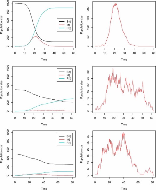
Stochastic SIR trajectories for susceptible S, infected I, and recovered R populations, with (top row) and , (middle row) and , and (bottom row) and . (The right column shows infected I only.)
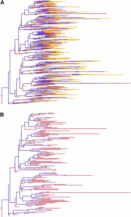
(A) Full stochastic SIR transmission tree with both sampled ψ-tips, shown in red, and otherwise removed μ-tips, shown in yellow. (B) The corresponding 140-tip sampled stochastic SIR tree. A and B were generated in FigTree (Rambaut 2007).
We required that the trees had leaves, filtering out those in which the epidemic died out in the early stages, i.e., when the initial infected individual was removed from the effective population too quickly to infect others. (Note that the inference procedures discussed in this article all implicitly condition on the number of leaves.) The probability that the first event in a given trajectory is the removal (by recovery, death, etc.) of patient zero is given by . When , this probability is . In our case, 52/152 () trees were “empty” or containing only one node. The filtering process left us with a mean of leaves for the simulated trees.
Homochronous trees:
A major concern in the comparison between Kühnert et al. (2014)’s birth–death-sampling SIR inference model, which includes explicit sampling, and our implementations of Volz (2012)’s coalescent SIR models, which do not include explicit sampling, is that the former is given extra information via the sampling process. Volz and Frost (2014) addressed this issue by providing a coalescent SIR model that does incorporate sampling explicitly.
That being said, results from Bošková et al. (2014) indicate that the poor performance of the deterministic coalescent SIR model in comparison with birth–death models was due to the lack of handling stochastic population size changes through time rather than the lack of information about the sampling proportion. Their results showed that the coalescent is “very robust to changes in sampling schemes” (Boskova et al. 2014, p. 8).
Regardless, to ensure a fair comparison of BDSIR and the coalescent SIR models, we simulated an SIR epidemic with homochronous, or contemporaneous, sampling. This type of simulation affords no additional information about the population size for explicit-sampling models, as there is only a single time of sampling.
We selected a simulation time of for the homochronously sampled trees, with the trajectories being sampled at high prevalence but also past the time of peak prevalence. This is important for distinguishing SIR from SI/SIS outbreaks, as it provides information about the removal parameter γ. In this set of simulations, each lineage was sampled at with probability 0.7 (the leaf count distribution for varied sampling probabilities is in File S1).
Simulated sequences:
To assess the ability of each SIR model to infer epidemic parameters with the inclusion of phylogenetic uncertainty, we also simulated the evolution of 2000-bp sequences down each simulated tree. We time stamped the sequences with the tip dates of each corresponding tree and informed the inference with the true Hasegawa–Kishino–Yano (HKY) substitution model (Hasegawa et al. 1985), clock rate , and . These choices were made to reflect real data, specifically those of influenza (Vaughan et al. 2014).
Along with simulated sequence data, analyses were performed with the simulated trees fixed (results are in File S1), and the parameters , γ, , and the origin of the tree were estimated with Bayesian prior distributions as listed in Table 4.
Deterministic coalescent SIR on higher and :
Finally, we had particular interest in the effects of varying the population size parameter on the deterministic coalescent SIR model, as comparisons from initial analyses with lower true (≈1.5 and ≈1.1) and (= 499) showed higher error and bias and lower 95% HPD coverage. Also, it is often assumed that deterministic descriptions will perform well for higher and larger population sizes. Table S7 and Table S9 detail the parameter values we used to explore the behavior of the deterministic coalescent on varied and combinations.
Interpretation of results
Results for simulated sequences: ,
| η | Inference | Truth | Mean | Median | Error | Bias | Relative HPD width | 95% HPD accuracy (%) |
|---|---|---|---|---|---|---|---|---|
| Stoch.Coal.SIR | 2.50 | 2.41 | 2.16 | 0.13 | −0.11 | 0.97 | 97.00 | |
| Deter.Coal.SIR | 2.50 | 2.78 | 2.03 | 0.38 | 0.05 | 0.79 | 87.00 | |
| BDSIR | 2.50 | 3.21 | 2.84 | 0.15 | 0.14 | 1.86 | 100.00 | |
| γ | Stoch.Coal.SIR | 0.30 | 0.16 | 0.13 | 0.52 | −0.52 | 0.82 | 47.00 |
| Deter.Coal.SIR | 0.30 | 0.25 | 0.16 | 0.56 | −0.28 | 0.97 | 56.00 | |
| BDSIR | 0.30 | 0.17 | 0.14 | 0.52 | −0.52 | 1.13 | 84.00 | |
| Stoch.Coal.SIR | 999 | 1805 | 1148 | 0.32 | 0.21 | 5.12 | 99.00 | |
| Deter.Coal.SIR | 999 | 2384 | 1565 | 0.66 | 0.60 | 6.54 | 100.00 | |
| BDSIR | 999 | 4002 | 2611 | 1.70 | 1.70 | 10.38 | 99.00 | |
| Stoch.Coal.SIR | Varies | 51.67 | 48.89 | 0.26 | 0.23 | 0.61 | 37.00 | |
| Deter.Coal.SIR | Varies | 49.13 | 46.46 | 0.22 | 0.20 | 0.26 | 29.00 | |
| BDSIR | Varies | 31.16 | 29.52 | 0.51 | 0.51 | 0.79 | 18.00 |
Simulation study results for fixed trees: and , and , and and
| η | Inference | Truth | Mean | Median | Error | Bias | Relative HPD width | 95% HPD accuracy (%) |
|---|---|---|---|---|---|---|---|---|
| Stoch.Coal.SIR | 2.50 | 2.84 | 2.68 | 0.12 | 0.09 | 0.98 | 100.00 | |
| Deter.Coal.SIR | 2.50 | 2.68 | 2.49 | 0.13 | 0.04 | 0.81 | 98.00 | |
| BDSIR | 2.50 | 2.73 | 2.67 | 0.12 | 0.08 | 0.55 | 94.00 | |
| γ | Stoch.Coal.SIR | 0.30 | 0.27 | 0.25 | 0.19 | −0.13 | 1.14 | 99.00 |
| Deter.Coal.SIR | 0.30 | 0.32 | 0.29 | 0.16 | 3.14E-3 | 1.27 | 99.00 | |
| BDSIR | 0.30 | 0.28 | 0.27 | 0.13 | −0.09 | 0.62 | 95.00 | |
| Stoch.Coal.SIR | 999 | 1390 | 921 | 0.19 | −0.03 | 3.85 | 100.00 | |
| Deter.Coal.SIR | 999 | 1807 | 1133 | 0.52 | 0.29 | 4.59 | 98.00 | |
| BDSIR | 999 | 1591 | 1142 | 0.39 | 0.24 | 3.42 | 99.00 | |
| Stoch.Coal.SIR | Varies | 41.81 | 40.35 | 0.03 | 0.01 | 0.20 | 99.00 | |
| Deter.Coal.SIR | Varies | 41.17 | 39.99 | 0.03 | 0.01 | 0.07 | 76.00 | |
| BDSIR | Varies | 40.89 | 39.72 | 8.65E-4 | −5.13E-4 | 3.43E-3 | 97.00 | |
| Stoch.Coal.SIR | 1.50 | 1.48 | 1.37 | 0.09 | −0.06 | 0.81 | 100.00 | |
| Deter.Coal.SIR | 1.50 | 1.80 | 1.49 | 0.24 | 0.15 | 0.52 | 85.00 | |
| BDSIR | 1.50 | 1.46 | 1.43 | 0.08 | −0.03 | 0.47 | 99.00 | |
| γ | Stoch.Coal.SIR | 0.30 | 0.19 | 0.17 | 0.40 | −0.40 | 1.06 | 85.00 |
| Deter.Coal.SIR | 0.30 | 0.26 | 0.23 | 0.27 | −0.22 | 1.15 | 89.00 | |
| BDSIR | 0.30 | 0.26 | 0.25 | 0.18 | −0.18 | 0.72 | 97.00 | |
| Stoch.Coal.SIR | 499 | 599 | 390 | 0.25 | −0.22 | 3.56 | 100.00 | |
| Deter.Coal.SIR | 499 | 562 | 361 | 0.44 | −0.26 | 3.36 | 91.00 | |
| BDSIR | 499 | 996 | 714 | 0.51 | 0.49 | 4.63 | 100.00 | |
| Stoch.Coal.SIR | Varies | 76.47 | 68.24 | 0.55 | 0.54 | 0.58 | 99.00 | |
| Deter.Coal.SIR | Varies | 91.03 | 72.51 | 0.39 | 0.38 | 0.42 | 88.00 | |
| BDSIR | Varies | 69.11 | 66.51 | 0.34 | −0.31 | 0.20 | 94.00 | |
| Stoch.Coal.SIR | 1.10 | 1.39 | 1.32 | 0.22 | 0.22 | 1.09 | 99.00 | |
| Deter.Coal.SIR | 1.10 | 1.68 | 1.44 | 0.46 | 0.46 | 0.59 | 25.00 | |
| BDSIR | 1.10 | 1.34 | 1.32 | 0.20 | 0.20 | 0.51 | 75.00 | |
| γ | Stoch.Coal.SIR | 0.25 | 0.17 | 0.15 | 0.37 | −0.36 | 1.11 | 84.00 |
| Deter.Coal.SIR | 0.25 | 0.22 | 0.18 | 0.30 | −0.22 | 1.16 | 86.00 | |
| BDSIR | 0.25 | 0.28 | 0.26 | 0.12 | 0.09 | 0.92 | 100.00 | |
| Stoch.Coal.SIR | 499 | 608 | 398 | 0.24 | −0.18 | 3.38 | 100.00 | |
| Deter.Coal.SIR | 499 | 553 | 337 | 0.42 | −0.26 | 3.08 | 92.00 | |
| BDSIR | 499 | 1471 | 1040 | 1.21 | 1.21 | 6.52 | 99.00 | |
| Stoch.Coal.SIR | Varies | 91.60 | 84.55 | 0.06 | 0.02 | 0.60 | 97.00 | |
| Deter.Coal.SIR | Varies | 112.79 | 90.37 | 0.26 | 0.26 | 0.94 | 85.00 | |
| BDSIR | Varies | 82.98 | 80.93 | 0.02 | −0.01 | 0.08 | 88.00 |
Epidemic parameter inference from H1N1 sequences in New Zealand
| Inference model | γ | Root of the tree (yr) | Origin of the epidemic (yr) | ||
|---|---|---|---|---|---|
| Stoch. Coal. SIR | 1.46 (1.04–2.14) | 27.08 (4.20–64.03) | 6.90E4 (175–2.86E5) | 0.53 (0.44–0.61) | 0.69 (0.45–1.03) |
| Deter. Coal. SIR | 1.35 (1.05–1.84) | 34.50 (3.86–82.16) | 1.20E5 (29–4.59E5) | 0.54 (0.45–0.62) | 0.73 (0.47–1.04) |
| BDSIR | 1.61 (1.09–2.29) | 27.72 (6.82–55.04) | 2.22E4 (259–9.38E4) | 0.49 (0.41–0.56) | 0.53 (0.43–0.65) |
Shown are mean estimates (and 95% HPD intervals) of each epidemic parameter inferred from seasonal influenza A (H1N1) sequence data collected in the Canterbury region of New Zealand throughout the 2001 flu season.
| Inference model | γ | Root of the tree (yr) | Origin of the epidemic (yr) | ||
|---|---|---|---|---|---|
| Stoch. Coal. SIR | 1.46 (1.04–2.14) | 27.08 (4.20–64.03) | 6.90E4 (175–2.86E5) | 0.53 (0.44–0.61) | 0.69 (0.45–1.03) |
| Deter. Coal. SIR | 1.35 (1.05–1.84) | 34.50 (3.86–82.16) | 1.20E5 (29–4.59E5) | 0.54 (0.45–0.62) | 0.73 (0.47–1.04) |
| BDSIR | 1.61 (1.09–2.29) | 27.72 (6.82–55.04) | 2.22E4 (259–9.38E4) | 0.49 (0.41–0.56) | 0.53 (0.43–0.65) |
Shown are mean estimates (and 95% HPD intervals) of each epidemic parameter inferred from seasonal influenza A (H1N1) sequence data collected in the Canterbury region of New Zealand throughout the 2001 flu season.
H1N1 data analysis
To test the efficacy of the coalescent SIR models on real data, epidemic parameters , γ, , and time of origin were estimated from 42 seasonal influenza A (H1N1) sequences sampled throughout the 2001 flu season in Canterbury, New Zealand.
Influenza infections are well known for their seasonal SIR behavior in nonequatorial populations, as each annual flu season begins with a supply of susceptible hosts and tapers off as the hosts recover with adaptive immunity (Iwasaki and Pillai 2014). Due partly to this seasonal pattern, the influenza virus is both a motivator for the development of specialized models and a prime subject for testing phylodynamic models (Koelle et al. 2006).
Sampling a particular region bypasses the necessity of specifying geographically structured populations, and New Zealand is an area of particular interest due to its geographic location and relative isolation from other regions with potentially varying dynamics. It is also assumed to play a key role in the global circulation of influenza strains (Rambaut and Holmes 2009; Bedford et al. 2010).
We used an HKY nucleotide substitution model, with a substitution rate of 5E-3 as estimated in Vaughan et al. (2014), and informed the models with dated sequences. Priors used for the Bayesian inference are shown in Table 4.
Bayesian prior distributions
| Annalysis | γ | ||||
|---|---|---|---|---|---|
| , | LogN(1, 1) | LogN(−1, 1) | LogN(7, 1) | Unif(0, 100) | Beta(1, 1) |
| , | LogN(0.5, 1) | LogN(−1, 1) | LogN(6, 1) | Unif(0, 500) | Beta(1, 1) |
| , | LogN(0.1, 1) | LogN(−1.5, 1) | LogN(6, 1) | Unif(0, 500) | Beta(1, 1) |
| , a | LogN(0.1, 1) | LogN(−1.5, 1) | LogN(7, 1) | Unif(0, 500) | — |
| , a | LogN(0.1, 1) | LogN(−1.5, 1) | LogN(7.5, 1) | Unif(0, 500) | — |
| , a | LogN(0.2, 1) | LogN(−1, 1) | LogN(6, 1) | Unif(0, 500) | — |
| H1N1 | Unif(0, 10) | LogN(3, 0.75) | LogN(13, 2) | Unif(0, 10) | Beta(1, 1) |
| HIV-1 | LogN(1, 1) | LogN(−1, 1) | LogN(7, 1) | Unif(0, 100) | Beta(1, 1) |
Shown are prior distributions for the reestimation of SIR parameters—the reproductive ratio , the rate of removal γ, the number of susceptible individuals at the start of the epidemic , the time of origin , and the sampling proportion for BDSIR—from the simulated trees, seasonal influenza A (H1N1), and human immunodeficiency virus (HIV-1) data analyses. LogN(M, S) is a log-normal distribution with mean M and standard deviation S in log space.
Only applies to deterministic coalescent SIR; see details in File S1.
| Annalysis | γ | ||||
|---|---|---|---|---|---|
| , | LogN(1, 1) | LogN(−1, 1) | LogN(7, 1) | Unif(0, 100) | Beta(1, 1) |
| , | LogN(0.5, 1) | LogN(−1, 1) | LogN(6, 1) | Unif(0, 500) | Beta(1, 1) |
| , | LogN(0.1, 1) | LogN(−1.5, 1) | LogN(6, 1) | Unif(0, 500) | Beta(1, 1) |
| , a | LogN(0.1, 1) | LogN(−1.5, 1) | LogN(7, 1) | Unif(0, 500) | — |
| , a | LogN(0.1, 1) | LogN(−1.5, 1) | LogN(7.5, 1) | Unif(0, 500) | — |
| , a | LogN(0.2, 1) | LogN(−1, 1) | LogN(6, 1) | Unif(0, 500) | — |
| H1N1 | Unif(0, 10) | LogN(3, 0.75) | LogN(13, 2) | Unif(0, 10) | Beta(1, 1) |
| HIV-1 | LogN(1, 1) | LogN(−1, 1) | LogN(7, 1) | Unif(0, 100) | Beta(1, 1) |
Shown are prior distributions for the reestimation of SIR parameters—the reproductive ratio , the rate of removal γ, the number of susceptible individuals at the start of the epidemic , the time of origin , and the sampling proportion for BDSIR—from the simulated trees, seasonal influenza A (H1N1), and human immunodeficiency virus (HIV-1) data analyses. LogN(M, S) is a log-normal distribution with mean M and standard deviation S in log space.
Only applies to deterministic coalescent SIR; see details in File S1.
HIV-1 data analysis
In addition to our analysis of H1N1 sequence data, we selected HIV-1 subtype B nucleotide sequences collected from infected individuals located in the United Kingdom. The coalescent SIR results were collated with the results from the BDSIR data analysis performed by Kühnert et al. (2014), using the same sequences. More details of this analysis are provided in File S1.
Results and Discussion
Simulation study
Results for epidemic parameter inference from nucleotide sequences simulated from stochastic SIR trees are provided in Table 1 for . Results for inference from fixed trees (, , ) are shown in Table 2, with 95% HPD coverage shown for each analysis in Figure 3. Inference results for analyses with true and varying population size () are described in Tables S1 and S2 in the supporting information, along with results from trees simulated under the stochastic and deterministic coalescent models for validation.
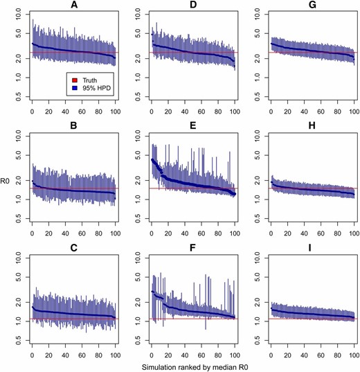
Estimates of from true stochastic SIR trees using inference methods by column, with stochastic coalescent SIR (A–C), deterministic coalescent SIR (D–F), and BDSIR (G–I). The truth varies by row, with (A, D, and G), (B, E, and H), and (C, F, and I).
Heterochronous trees:
For , all three inference methods performed similarly for parameters and γ, with high 95% HPD coverage and low error and bias. The most weakly identifiable parameter yielded the largest HPD intervals for all three inference models. The deterministic coalescent returned higher error (0.52) and bias (0.29) than the stochastic coalescent SIR (0.19, −0.03) and BDSIR (0.39, 0.24) and recovered the origin parameter for only 76 of 100 simulated trees, while the stochastic coalescent and BDSIR respectively recovered for 99 and 97 of 100 simulations.
For , the relative HPD widths (akin to variance) for three of the four estimated parameters (, γ, and ) were smallest for BDSIR. For the parameter , the relative HPD width is largest for BDSIR, although it also had slightly higher 95% HPD coverage than deterministic coalescent SIR and the same as stochastic coalescent SIR. The deterministic coalescent SIR method recovered the truth for 85, 89, 91, and 88 of 100 trees for parameters , γ, , and , while its stochastic analog recovered the truth for 100, 85, 100, and 99 of 100 trees for the same parameters. Finally, for stochastic coalescent SIR and BDSIR, error and (absolute) bias were relatively low for , arguably the parameter of most interest to epidemiologists since it represents the number of individuals each infected individual will infect in a naive population. Deterministic coalescent SIR has a higher error (0.24) and bias (0.15) and also has significantly lower coverage for (85%).
For , the two stochastic models again outperformed the deterministic coalescent in error, bias, and 95% HPD coverage. The stochastic coalescent most reliably recovered the truth for (99 of 100 simulations), while the deterministic coalescent had more than double the error and bias and still recovered the truth for only 25 of the 100 simulations. BDSIR had the lowest error and bias for under this scheme, although it recovered the truth for only 75 of 100 simulations. For removal parameter γ, BDSIR again yielded lower error and bias, in this case returning the truth for 100/100 trees (in contrast to 84 and 86 from the stochastic and deterministic coalescent, respectively).
In the stochastic models, there is a greater trade-off between parameters due to the impact the relationship between them has on the survival of trajectories at low . A larger estimated removal rate tends to require a larger susceptible population for the epidemic to avoid dying out in the early stages. Likewise, a smaller susceptible population implies a smaller estimated γ.
Deterministic coalescent SIR on higher and :
As mentioned in the preceding subsection, the deterministic coalescent model yielded higher error and bias than both the stochastic coalescent and BDSIR for most parameters with and .
To investigate the deterministic model’s sensitivity to population sizes, we also simulated a range of population sizes ( 499, 999, and 1999) for . Even with , the deterministic coalescent SIR model’s 95% HPD coverage was low. For parameters , γ, , and , this coverage was respectively 40%, 64%, 66%, and 18%. Table S6 shows these results.
Additionally, we increased both (to 3.5 and 5) and (to 4999 and 9999). However, for parameters , γ, and , the deterministic coalescent SIR showed increased error, bias, and HPD widths, and the HPD coverage for did not improve. These results are shown in Table S9.
While each of these methods is an approximation, the deterministic coalescent particularly suffers from model misspecification since it does not account for the stochasticity that is always present in the early stages of epidemics, regardless of .
Homochronous trees:
Results for homochronously sampled trees are given in Table S3.
All three SIR inference models recover the truth for >95/100 trees within their respective 95% HPD widths for epidemic parameters , γ, and . The time of origin was recovered for 100/100 trees by BDSIR, 95/100 trees by stochastic coalescent SIR, and 73/100 trees by deterministic coalescent SIR. However, relative error and bias also increased consistently across all three models, along with the 95% HPD widths. The deterministic coalescent had the highest error, bias, and HPD width for and highest error and HPD width for , which is consistent with the heterochronously sampled data.
Further consideration of the effects of sampling rate changes and sampling model misspecification are warranted for BDSIR and coalescent SIR, the latter of which has been facilitated by Volz and Frost (2014).
Simulated sequences:
Relative error and bias were inflated across all three inference models with the addition of phylogenetic uncertainty, and in certain cases the 95% HPD coverage was lower than with fixed trees. The deterministic coalescent model recovered the truth within its 95% HPD intervals only for ≥90 of the 100 trees in the case of . The true values for the parameters , γ, and were covered by 95% HPD intervals for 87, 56, and 29 of the 100 trees, respectively. This is contrasted with the performance of the stochastic coalescent (100, 97, 47, and 37 for parameters , , γ, and ) and BDSIR (99, 100, 84, and 18 for , , γ, and ), as shown in Table 1.
Error, bias, and 95% HPD widths were higher with simulated sequences for all three inference models for parameters γ, , and than with fixed trees. This indicates the importance of calibrating epidemic parameters of interest. In our case, we emphasize the basic reproductive number , often the parameter of most interest to epidemiologists. For , stochastic coalescent SIR and BDSIR recovered the truth within their 95% HPD intervals for 97 and 100 of the 100 simulations, respectively. They also showed only slight changes in error and bias compared to inference performed on the fixed trees used to generate the sequences. The deterministic coalescent SIR model recovered for 87 of the 100 simulations (contrasted with 98/100 for the fixed trees) and with increased error.
Priors and identifiability:
It is important to understand the impact of selected priors on inference results, as the priors are where the power of Bayesian inference lies. For example, we found relatively weak identifiability in the initial susceptible population parameter , which must either be fixed or be estimated alongside the origin parameter .
In addition to allowing each parameter to be either fixed or estimated, we have provided options for parameterization of our models, with either the transmission rate β or acting as operable parameters in MCMC analysis. For the deterministic coalescent, there is also an option to use the intrinsic growth parameter described by Dearlove and Wilson (2013).
The choice of parameterization necessarily affects the prior that will be used in the inference and should be considered carefully. However, we found that once a parameterization has been selected, our inference models are robust to different prior distributions placed on each parameter. We also used broader prior distributions on the deterministic coalescent to test whether this would increase its lower 95% HPD coverage relative to the stochastic models. We found that doing so increased the error and bias of the results without increasing the accuracy (shown in Table S4).
H1N1 data analysis
Epidemic parameter estimates from serially sampled influenza A (H1N1) virus sequence data are shown in Table 3.
The estimated means of the basic reproductive number were 1.46, 1.35, and 1.61 for the stochastic coalescent, the deterministic coalescent, and BDSIR, respectively. Estimates of from pandemic H1N1 in New Zealand range from ∼1.2 to 1.5 (Paine et al. 2010; Opatowski et al. 2011; Roberts and Nishiura 2011; Roberts 2013; Biggerstaff et al. 2014), and estimates of for seasonal H1N1 from other countries also range from ∼1.2 to 1.5 (Chowell et al. 2008). The 95% HPD intervals were very similar across each model, ranging from just over 1.0 to ∼2.0.
The population of the Canterbury region in 2001 was reported to be ∼481, 431 by the Environment Canterbury Regional Council (Ecan 2001) and 521, 832 by Statistics New Zealand (StatsNZ 2001). The mean estimates of were considerably lower using the stochastic coalescent (), the deterministic coalescent (), and BDSIR (). However, the effective population of susceptibles is assumed to be much smaller, as the total population contains individuals of various susceptibility, e.g., those with partial immunity from vaccination and previous or secondary infections.
Most people recover from flu symptoms, the time they are likely to be most infectious, within a few days up to 2 weeks (CDC 2014; WHO 2014). This provides a range of probable true values for the removal parameter γ. The sequence data and molecular clock rate, and therefore the tree, are in units of years. Therefore, our γ range would be from 365/14 days to 365/2 days or from to . The stochastic coalescent, the deterministic coalescent, and BDSIR respectively inferred γ means of 27.08, 34.50, and 27.72. These estimates are on the low side compared to epidemiological models for influenza that include explicit spatial and household effects (Ferguson et al. 2005), but a moderate misfit of the model is not unexpected when fitting a simple closed SIR model with no population substructure.
The root of the tree was very similar across all inference models, respectively 0.53, 0.54, and 0.49 for stochastic coalescent SIR, deterministic coalescent SIR, and BDSIR. The same was true for the origin , with: 0.69, 0.73, and 0.53 for the stochastic coalescent, the deterministic coalescent, and BDSIR. All three inference models returned tree root and origin estimates that are consistent with previous estimates from single flu seasons. That is, the tree age is young and the root coincides with the start of the (winter) influenza season in the Southern Hemisphere. The time of introduction of influenza into the region, , was 1 or 2 months before the root. This supports the notion that the sequences selected represent a single introduction of the strain into the Canterbury population (see File S1 for details of data selection and Figure S4 for representative trees inferred from an alternate data selection.).
The trees estimated by each of the three models are typical for influenza (see Figure 4 for representative trees from each posterior), with branches that are quick to coalesce moving backward in time from the most recently sampled tip.
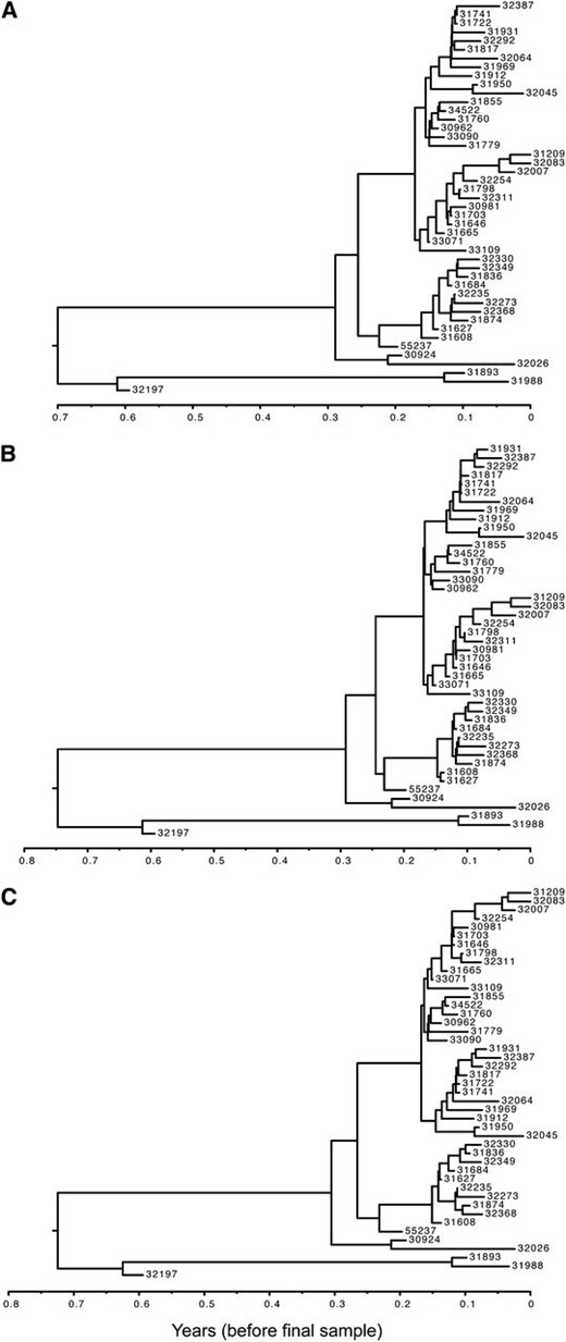
Representative influenza A (H1N1) posterior trees from inference using the (A) BDSIR, (B) stochastic coalescent SIR, and (C) deterministic coalescent SIR inference models.
HIV-1 data analysis
Results for inference from HIV-1 sequence data can be found in File S1. 95% HPD intervals are shown in Figure S5, Figure S6, Figure S7, and Table S8.
Computational efficiency
Finally, Table S5 shows comparisons of computation times under each inference model for each type of data analyzed. The deterministic coalescent SIR model is by far the fastest to sample and converge, with stochastic coalescent SIR and BDSIR varying, depending on the type of data.
Closing remarks
A key reason for the success of coalescent theory in population genetics is its mathematical simplicity and the computational efficiency of calculating the probability density of a sample genealogy. Our results show that a stochastic variant of coalescent theory can be successfully adapted to estimate epidemiological parameters in a true Bayesian inference context. This stochastic coalescent SIR model performs better than the deterministic analog for estimating epidemic parameters in some circumstances. Unfortunately, the stochastic model relies on a computationally demanding Monte Carlo estimate of the coalescent density via simulation of an ensemble of epidemic trajectories, negating one of the main advantages of coalescent theory. In fact, the current implementation is less computationally efficient than the implementation of the BDSIR model. However, an advantage of the stochastic coalescent over the explicit sampling model in BDSIR is its robustness to biased sampling schemes, as has been shown for the case of pure exponential growth dynamics (Bošková et al. 2014).
A more computationally efficient approach to computing the coalescent probability of the sample genealogy in the stochastic setting would be to use particle filtering (Andrieu and Roberts 2009; Andrieu et al. 2010; Rasmussen et al. 2011, 2014), but there are no theoretical barriers to applying particle MCMC to the exact model (Stadler et al. 2014). Therefore, an obvious extension of this work would be to apply particle MCMC algorithms to the exact stochastic SIR model that was used in simulations in this work. We anticipate that the exact model would outperform all the methods tested here, especially when is close to one.
In the meantime, the Bayesian coalescent inference methods developed here make it feasible to estimate epidemic parameters from time-stamped, serially sampled molecular sequence data, while accurately accounting for uncertainty in the topology and the divergence times of the phylogenetic tree.
Acknowledgments
We thank Gabriel Leventhal and Louis Du Plessis (ETH Zürich) for constructive and valuable input and the New Zealand eScience Infrastructure for access to high-performance computing facilities (http://www.nesi.org.nz/). A.J.D. was funded by a Rutherford Discovery Fellowship from the Royal Society of New Zealand. A.P., T.V., T.S., and A.J.D. were also partially supported by Marsden grant UOA1324 from the Royal Society of New Zealand (http://www.royalsociety.org.nz/programmes/funds/marsden/awards/2013-awards/).
Footnotes
Supporting information is available online at http://www.genetics.org/lookup/suppl/doi:10.1534/genetics.114.172791/-/DC1.
Available freely online through the author-supported open access option.
Communicating editor: Y. S. Song
Literature Cited
CDC, 2014 United States Centers for Disease Control and Prevention. Available at: http://www.cdc.gov/flu/. Accessed: November, 2014.
ECAN, 2001 Environment Canterbury Regional Council. Available at: http://ecan.govt.nz/about-us/population/how-many/pages/census.aspx. Accessed: November, 2014.
Gavryushkina, A., D. Welch, T. Stadler, and A. Drummond, 2014 Bayesian inference of sampled ancestor trees for epidemiology and fossil calibration. arXiv:1406.4573.
Kermack, W., and A. McKendrick, 1932 Contributions to the mathematical theory of epidemics. ii. The problem of endemicity. Proc. R. Soc. A 138: 55–83.
Paine, S., G. Mercer, P. Kelly, D. Bandaranayake, M. Baker et al., 2010 Transmissability of 2009 pandemic influenza a(h1n1) in New Zealand: effective reproduction number and influence of age, ethnicity, and importations. Eurosurveillance 15(24). Available at: http://www.eurosurveillance.org/ViewArticle.aspx?ArticleId=19591.
Rambaut, A., 2007 Figtree. Available at: http://tree.bio.ed.ac.uk/software/figtree/.
Rodrigo, A., and J. Felsenstein, 1999 Coalescent approaches to HIV population genetics, pp. 233–272 in The evolution of HIV, edited by K. A. Crandall. The Johns Hopkins University Press, Baltimore.
Stadler, T., T. G. Vaughan, A. Gavruskin, S. Guindon, D. Kühnert, et al., 2014 Population genetics vs. population dynamics: How well can coalescent-based models approximate population dynamic processes? Genetics 190: 187–201.
StatsNZ, 2001 Statistics New Zealand. Available at: http://stats.govt.nz/Census/.
Vaughan, T., D. Kühnert, A. Popinga, D. Welch, and A. Drummond, 2014 Efficient Bayesian inference under the structured coalescent. Bioinformatics 30: 2272–2279.
WHO, 2014 World Health Organization. Available at: http://www.who.int/topics/influenza/en/. Accessed: November, 2014.
