


Abstract
Frequency-dependent selection (FDS) remains a common heuristic explanation for the maintenance of genetic variation in natural populations. The pairwise-interaction model (PIM) is a well-studied general model of frequency-dependent selection, which assumes that a genotype’s fitness is a function of within-population intergenotypic interactions. Previous theoretical work indicated that this type of model is able to sustain large numbers of alleles at a single locus when it incorporates recurrent mutation. These studies, however, have ignored the impact of the distribution of fitness effects of new mutations on the dynamics and end results of polymorphism construction. We suggest that a natural way to model mutation would be to assume mutant fitness is related to the fitness of the parental allele, i.e., the existing allele from which the mutant arose. Here we examine the numbers and distributions of fitnesses and alleles produced by construction under the PIM with mutation from parental alleles and the impacts on such measures due to different methods of generating mutant fitnesses. We find that, in comparison with previous results, generating mutants from existing alleles lowers the average number of alleles likely to be observed in a system subject to FDS, but produces polymorphisms that are highly stable and have realistic allele-frequency distributions.
IT has been nearly 50 years since molecular techniques first revealed the ubiquity of genetic variation in nature (Hubby and Lewontin 1966). Neutral theories of the maintenance of variation (Ohta 1973; Kimura 1984) remain the dominant framework underlying most population-genetic models, but we now know that most, if not all, genetic variation is subject to some degree of natural selection (Hahn 2008). Despite a rich theoretical and empirical literature on the subject, however, pinning down the mechanisms that allow selective maintenance of genetic variation remains a stubborn challenge (Leffler et al. 2012).
Early theoretical work in this area focused on the maintenance of diallelic polymorphisms (e.g., Levene 1953; Li 1955; Lewontin 1958; Haldane and Jayakar 1963; Hedrick 1986), largely for mathematical convenience. Unfortunately, the results of diallelic approaches quite often do not scale up to the multiallelic case in intuitive or analytically tractable ways (Gillespie 1977; Lewontin et al. 1978; Karlin 1981; Clark and Feldman 1986; Matessi and Schneider 2009; Muirhead and Wakeley 2009; Nagylaki 2009; Schneider 2009; Waxman 2009). Empirical studies confirm that nonneutral polymorphisms with more than two alleles are very common (Keith 1983; Keith et al. 1985; Bradley et al. 1993; Moriyama and Powell 1996; Hahn 2008). MHC loci, to name one extreme example, can have hundreds of alleles (for a review, see Garrigan and Hedrick 2003).
The standard approach to modeling the maintenance of selected polymorphism—what we call the “parameter-space approach”—has been to generate large numbers of fitness sets, either randomly (Lewontin et al. 1978; Clark and Feldman 1986; Asmussen and Basnayake 1990; Gimelfarb 1998) or using some preselected patterns (Karlin 1981), to systematically search the available parameter space to assess which selection regimes and what proportion of parameter space maintain variation for a given number of alleles. This proportion is interpreted as an estimate of the “potential” for variation under a given selection regime. These types of models have typically found that the proportion of randomly generated fitness sets that maintain variation becomes vanishingly small for n > 5 alleles if viability is assumed to be constant (Gillespie 1977; Lewontin et al. 1978); the same holds true in models of constant fertility selection (Clark and Feldman 1986).
It is far more biologically reasonable to expect selection pressures to change in space or time, however (Kojima 1971). Modern hypotheses to explain selective polymorphism have included heterozygote advantage (e.g., Kekäläinen et al. 2009; Spurgin and Richardson 2010; Sellis et al. 2011), spatially heterogeneous selection (e.g., Hedrick 1986; Star et al. 2007a,b; Nagylaki 2009), and sexual antagonism (Curtsinger et al. 1994; Foerster et al. 2007; Hall et al. 2010; Mokkonen et al. 2011; Connallon and Clark 2012). Nevertheless, the most common heuristic invoked to explain nonneutral variation in natural systems remains frequency-dependent selection (FDS) (see Sinervo and Calsbeek 2006 for a review).
FDS describes any selection regime where a genotype’s fitness depends on the frequencies of its own or other genotypes in the population. Negative frequency dependence (selection in favor of rare alleles) is often invoked to explain polymorphism, since if it is beneficial to be rare, it is also difficult to go extinct. Conversely, positive frequency dependence (selection in favor of common alleles) is expected to eliminate variation. It is important to note that simple positive FDS and negative FDS are extremes at opposite ends of a continuum. Intraspecific interactions such as mate choice (e.g., Hughes et al. 1999) and alternative mating strategies (Sinervo and Lively 1996) have been shown to produce both negative and positive FDS, sometimes both within the same population (see Sinervo and Calsbeek 2006 for a review). Interspecific interactions such as mimicry (e.g., Borer et al. 2010), host–parasite coevolution (Dybdahl and Lively 1998; Koskella and Lively 2009), and predator–prey dynamics (e.g., Olendorf et al. 2006; Marples and Mappes 2010) can produce negative FDS, positive FDS, and other more nuanced FDS regimes. The diversity of FDS regimes observed in nature suggests that any investigation of the potential for genetic variation under FDS should use a very general model.
Here we restrict ourselves to the study of FDS that results from intraspecific interactions. The most general model of this kind of FDS is the discrete-time pairwise-interaction model (PIM) (Cockerham et al. 1972), which parameterizes fitness as a product of intraspecific competition at the genotype level. This approach provides a biologically reasonable way to model frequency-dependent viabilities, conceptually similar to the payoff matrix of evolutionary game-theoretic models (Maynard Smith 1982). The wildcard model of FDS (Matessi and Schneider 2009 and references therein) is a continuous-time analog to the PIM in the specific case of symmetric fitness interactions. The wildcard model leads to several useful results for multiple alleles (see Schneider 2009), but the requirement of symmetric interactions limits its generality. We are interested in exploring the full parameter space of frequency-dependent selective scenarios, and for our purposes the discrete-time PIM provides the most general framework available.
In the PIM each genotype is assumed to have a constant interaction fitness with every other genotype in the population. Assuming random mixing of individuals, the frequencies of interactions are given by the product of the frequencies of the interacting genotypes, and the total fitness of a genotype is a weighted sum of its fitnesses in interactions with all genotypes. This general formulation allows the PIM to parameterize a wide range of FDS regimes (positive, negative, balancing, and disruptive), as well as constant selection as a special case. A recent investigation of the potential for polymorphism under the PIM, using the parameter-space approach, found that FDS has a higher potential for variation than the equivalent constant viability model for any given number of alleles (Trotter and Spencer 2007). It was also found that a wide variety of flavors of FDS, not simply negative FDS, have potential for polymorphism under the PIM.
The traditional parameter-space approach, while informative, ignores the process of mutation and invasion that necessarily underlies the development of any natural polymorphism. An alternative, the so-called “constructionist” approach to modeling the maintenance of genetic variation, is analogous to some models of ecological community construction (Nee 1990). In a constructionist model, polymorphisms (communities) develop from monomorphisms (single species). New mutant alleles (species) are introduced at a set rate of mutation (migration) and allowed to invade or be repulsed by the existing system based on their relative fitnesses. Early constructionist models of genetic variation found that constant viability can easily generate intermediate numbers of alleles (Spencer and Marks 1988, 1992; Marks and Spencer 1991). A recent model of polymorphism construction using the PIM (Trotter and Spencer 2008) found FDS with recurrent mutation can result in very high levels of single-locus polymorphism.
A defining feature of this last model was the assumption that new mutant interaction fitnesses be drawn from a uniform distribution on [0, 1]. However, this method ignores the reality that new mutations result from changes (usually small) to an existing allele. This relationship suggests a more natural way to model mutants arising from within the population might be to have mutant fitnesses be some function of the fitness of a “parental” allele from which they descend. Because the vast majority of new mutations are neutral or weakly deleterious (Eyre-Walker and Keightley 2007), simulated mutants should be on average similar to, but less fit than, their parental allele. The model of Spencer and Marks (1992) incorporated mutation from existing alleles (parental allele, Ap, mutated to a novel allele, Am) in a constructionist approach to modeling the maintenance of variation by constant viability selection. In their models, the viabilities of mutant AiAm genotypes (wim) were drawn from distributions centered just below the fitness of the equivalent parental genotype AiAp (wip); hence most mutants were slightly deleterious. In this study, we incorporate mutation from existing alleles into constructionist approaches, using the PIM of FDS.
Models
We model selection acting on a large, isolated, randomly mating monoecious population of diploid organisms with nonoverlapping generations. Under the PIM, each genotype AiAj has constant fitnesses (wij,kl) in its interactions with the other genotypes AkAl in the population (i, j, k, l = 1, 2, …, n). These interaction fitnesses collectively define the fitness set. We assume AiAj is equivalent to AjAi, and so wij,kl = wji,kl = wij,lk = wji,lk.
When adding a new allele to an n-allele system with PIM fitnesses, there are several different types of interactions that need to be parameterized and (n + 1)3 new interaction fitnesses that must be generated. This extra dimension of fitness makes linking mutant fitnesses to a parental allele a more complicated endeavor. The addition of a new allele, An+1, results in n + 1 new genotypes, each of which must be assigned interaction fitnesses for their interactions with the existing genotypes and the n + 1 new genotypes. We refer to these interaction fitnesses as the mutant fitnesses. In addition, each existing genotype must also be given n + 1 new interaction fitnesses, corresponding to their interactions with each of the new genotypes. We refer to these as the mutant impacts, as they represent the change to the fitnesses of existing genotypes due to their interactions with the new mutant. The number of elements in the updated fitness set, the sum of the number of mutant fitnesses and impacts therefore, is
We use four separate cases of the PIM construction model, as detailed below, to investigate the consequences of different methods of generating mutant fitnesses and mutant impacts. The first two cases illustrate the effects of generating mutant fitnesses related to a given existing allele’s fitnesses. The second pair of cases illustrates the additional changes in model behavior resulting from generating mutant impacts related to the existing impacts of a given parental allele. For all cases, we are interested in the levels and stability of polymorphism and distributions of fitness produced by construction under the PIM with mutation from existing alleles and the impacts on such measures due to the different methods of generating fitnesses.
The constructionist approach to modeling selection has three stages each generation: mutation, selection, and extinction check.
Mutation
Every generation, an allele existing in the population is chosen to mutate. (For the effects of different mutation rates, see File S1.) The probability of a given allele (Ai) being chosen as a “parent” allele is proportional to its frequency in the population, pi. The frequency of the parental allele (Ap) is then decremented by 10−6 and the mutant allele (Am, where m = n + 1) is introduced at frequency of 10−6. We assume this implied population size of N = 5 × 10⁵ is large enough to ignore the effects of random drift. New interaction fitnesses are added to the fitness set in three stages. First, the preexisting genotypes (AiAj) are assigned fitnesses in their interactions with the new mutant genotypes (AkAm). These fitnesses, wij,km, represent the “impact” of the new mutant on the fitness of existing genotypes. Second, the new mutant genotypes are assigned fitnesses in their interactions with the preexisting genotypes, wkm,ij. Finally, the mutant genotypes are assigned fitnesses in their interactions with the other mutant genotypes, wim,km.
We investigated five different methods for generating the required new interaction fitnesses after the addition of mutant alleles. A summary of the methods of generating fitnesses used in each case can be found in Table 1.
Guide to the cases of the PIM
| Case | wij,km (existing vs. mutant) | wkm,ij (mutant vs. existing) | wkm,im (mutant vs. mutant) |
|---|---|---|---|
| 0 | U[0, 1] | U[0,1] | U[0, 1] |
| 1 | U[0, 1] | αkp,ijwkp,ij | αkp,ipwkp,ip |
| 2 | U[0, 1] | αkp,ijwkp,ij, where k ≠ m | αkp,ipwkp,ip, where k ≠ m |
| βpp,ijwpp,ij, where k = m | βpp,ipwpp,ip, where k = m | ||
| 3 | wij,kp | αkp,ijwkp,ij | αkp,ipwkp,ip |
| 4 | αij,kpwij,kp | αkp,ijwkp,ij | αkp,ipwkp,ip |
General case
In the general form of the model, hereafter referred to as case 0, all new interaction fitnesses are drawn from the uniform distribution on [0, 1]. This method implies independence between the fitnesses of the parental and mutant alleles and the impact of the new allele on existing genotypes. The data shown for this case are taken from Trotter and Spencer (2008) and are used as the basis for comparison for the other cases.
Case 1
Empirical data suggest that the majority of new mutations are slightly deleterious (Mukai et al. 1966; Eyre-Walker and Keightley 2007). Consequently, in all further cases we model mutant fitnesses (wkm,ij) to be, on average, slightly lower than the equivalent parental fitness. In this first case of mutation from existing alleles, we continue to draw the wij,km impacts from the uniform distribution on [0, 1]. Each new mutant interaction fitness (wkm,ij), however, is now a function of the existing interaction fitness (wkp,ij) of the corresponding parental genotype (AkAp) and is given by αkp,ijwkp,ij. We draw the α from a rescaled beta-distribution on [0, 1.5] that is conditioned to have mean μα and variance σ2α. Note that a new, independent, α is drawn for every new mutant interaction fitness. For all our cases, we set 0 < μα < 1 and assume σ2α to be small. By rescaling the distribution of α in this way, we avoid negative fitnesses, but beneficial mutations (α > 1) remain possible but rare. In case 1, we set μα = 0.95, σ2α = 0.001, to produce primarily mutations of moderately negative effect, with rare beneficial mutations (<5%). (For details of the effects of varying μα and σ2α see File S1.)
We set homozygous mutants AmAm to be lethal with probability 0.05. (Interestingly, it turns out that models omitting this rare lethality produce nearly identical outcomes of polymorphism construction; see File S1.) In the case of lethality, all wmm,ij = 0; otherwise homozygote fitnesses are generated using the same method for all other wkm,ij.
Case 2
A previous model of mutation from existing alleles (Spencer and Marks 1992) assumed that heterozygote and homozygote fitnesses are drawn from slightly different distributions (with heterozygotes being, on average, fitter than homozygotes). For purposes of direct comparison with that model, we here recreate it using our PIM approach. We continue to draw the wij,km impacts from the uniform distribution on [0, 1]. Each mutant interaction fitness (wkm,ij) is a function of the existing interaction fitness (wkp,ij) of the corresponding parental genotype (AkAp) and is given by αkp,ijwkp,ij, where each α is drawn from a rescaled beta-distribution on [0, 1.5] with for heterozygotes (i.e., when k ≠ m), and by βkp,ijwkp,ij, where each β is drawn from a rescaled beta-distribution on [0, 1.5] with for homozygotes (i.e., when k = m).
Case 3
In this case, as in case 1, both homozygote and heterozygote mutant fitnesses are functions of the existing interaction fitness (wkp,ij) of the corresponding parental genotype (AkAp) and are given by αkp,ijwkp,ij, where each α is drawn from a rescaled beta-distribution on [0, 1.5] with . We know from the general construction PIM for FDS (Trotter and Spencer 2008) that the impacts, the wij,km, greatly affect the likelihood of allele Am successfully invading the polymorphism. A mutant allele that leads to low values of wij,km will drag down the fitnesses of existing alleles, thereby improving its own chances of invading the polymorphism. In this case, instead of drawing the wij,km from the uniform distribution, we assume the wij,km are strictly equal to the impacts of the parental allele wij,kp.
Case 4
In this case, instead of the wij,km being strictly equal to the equivalent parental fitness, we assume they have, on average, a slightly deleterious effect on existing genotypes. This deleterious effect is accomplished by setting all new interaction fitnesses as functions of the existing interaction fitness (wkp,ij) of the corresponding parental genotype (AkAp) and is given by αkp,ijwkp,ij, where each αijk is drawn from a rescaled beta-distribution on [0, 1.5] with . As a result, this case produces mutant alleles that have low fitness, but that are also good invaders. This case is motivated less by biological realism (we know of no reason to expect mutations to be biased in favor of negative impacts in this way) and more as a test of whether a mutant’s fitnesses, or its impact on other genotypes, are more important to invasion success.
Selection and extinction
Each model run was initialized with a single allele with fitness . Each generation we recorded the numbers, ages, and frequencies of all alleles and also the mean fitness. After 10,000 such generations had passed, we recorded fitness sets, as well as numbers and frequencies of alleles. Since FDS construction systems do not converge to a steady state (see Trotter and Spencer 2008), we wanted to run the mutation process for long enough to avoid sampling during the initial transient period, but not so long that assuming selection to be consistent for that many generations is unreasonable. The mutation process was halted after 10,000 generations and the system was allowed to continue iterating to equilibrium (defined as either a monomorphic equilibrium or a polymorphic equilibrium with |Δpi| < 10−8 for all i). At equilibrium, final measurements of the numbers, ages, and frequencies of alleles and the mean fitness were recorded. The equilibrium statistics indicate how much of the “snapshot” variation is transient and how much is likely to be permanent, as well as providing a means of comparing the results of the construction approach with those of earlier parameter-space approaches. For each case, 1000 replicate runs, differing only in the pseudorandom number seed, were performed.
Results
Allele numbers
Distributions of numbers of alleles present at snapshot and at equilibrium for all cases are shown in Figure 1, and summary statistics for these distributions are found in Table 2.
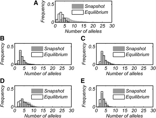
Numbers of alleles present at snapshot (shaded) and at equilibrium (open) in 1000 runs each for all cases of PIM construction. A–E represent cases 0–4 in order.
Summary statistics for numbers of alleles present at snapshot and equilibrium taken across 1000 runs each of all cases of PIM
| Minimum | Mean | Maximum | Variance | |||||
|---|---|---|---|---|---|---|---|---|
| Case | Snapshot | Equilibrium | Snapshot | Equilibrium | Snapshot | Equilibrium | Snapshot | Equilibrium |
| 0 | 1 | 1 | 7.4 | 3.4 | 31 | 9 | 17.378 | 1.883 |
| 1 | 2 | 1 | 4.853 | 3.811 | 25 | 19 | 9.9093 | 3.4507 |
| 2 | 1 | 1 | 4.83 | 4.051 | 27 | 20 | 7.2063 | 3.0134 |
| 3 | 2 | 2 | 5.983 | 4.651 | 15 | 13 | 5.274 | 4.0913 |
| 4 | 2 | 1 | 3.913 | 3.314 | 23 | 9 | 2.7442 | 1.1966 |
In all cases, the model produced an initial transient increase and subsequent crash in n, followed by perpetual fluctuations (Figure 2). In all cases, at least 99% of runs had ≥2 alleles at snapshot, while at equilibrium monomorphism was rare but possible (0.1–3% of runs). Case 4 produced snapshot polymorphisms with smallest average n (3.9 alleles), which is unsurprising since its mutation process draws all new interactions from distributions centered below the mean of existing fitnesses. Case 1 generated on average more alleles than case 2, despite case 2 having built-in heterozygote advantage. This trend is counter to the intuitive idea that, all else being equal, heterozygote advantage promotes polymorphism. Case 3 typically generated snapshot polymorphisms with the most alleles (∼6 on average).
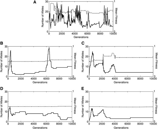
Time series data for numbers of alleles (n, thick solid line) and mean fitness (, dashed line) for randomly selected sample runs of all five cases with mutation from parental alleles. A–E represent cases 0–4 in order.
Mean fitness
Examples of the trajectories of mean fitness and allele number from all cases are illustrated in Figure 2. Each case occasionally (but rarely) produced fluctuating mean fitness trajectories such as those shown in Figure 3. During these fluctuations, while n remains constant the mean fitness decreases to some threshold, at which point multiple invasions occur and the mean fitness rebounds. A sharp spike in mean fitness often coincides with multiple extinctions as a highly fit allele drives others out.
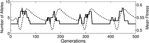
Close-up of an example of mean fitness oscillations from case 3 data. Cases 1–4 all occasionally produce these kinds of qualitatively repetitive dynamics.
Potential for polymorphism
The potential for polymorphism has been defined as the proportion of random initial allele frequencies and fitness sets that maintain all alleles under a given model (Lewontin et al. 1978; Asmussen and Basnayake 1990; Asmussen et al. 2004; Star et al. 2007a; Trotter and Spencer 2007, 2008). In the context of construction approaches, we measure potential as the proportion of model runs that maintained all alleles present at snapshot, at equilibrium. All four mutation-from-existing-alleles cases had a higher proportion of runs maintain all snapshot alleles than did the general case (see Figure 4). We see in Figure 4 that cases 3 and 4 appear to have slightly lower potential than cases 1 and 2 as n increases. Case 2 had an unusually large number of runs (83), maintaining six alleles at equilibrium.
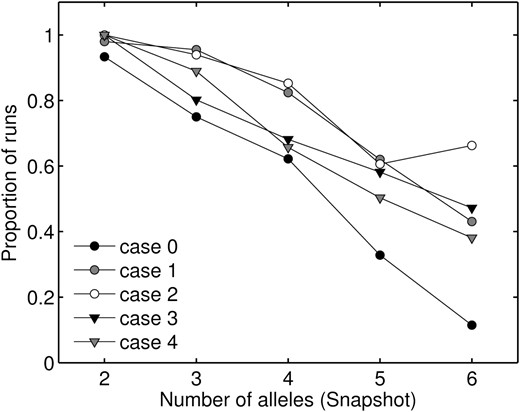
Proportion of fitness sets, from all variations on the PIM, that maintained all snapshot alleles at equilibrium, starting from the snapshot allele-frequency vector.
Another method of measuring the potential for variation is to iterate each snapshot fitness set to equilibrium from many starting allele-frequency vectors (Star et al. 2007b). The proportion of vectors that maintain all snapshot alleles for a particular fitness set gives a measure of the domain of attraction of the fully polymorphic equilibrium for that set. Star et al. (2007b) used this method to partition their equilibrium fitness sets into three classes: type I fitness sets maintain full polymorphism from all initial conditions and can be considered to have globally stable equilibria; type II fitness sets maintain all alleles from only a subset of all start vectors and thus have locally stable equilibria; and type III fitness sets lose at least one allele from all initial conditions, implying that some of the snapshot polymorphism is always transient. Numbers of type I, II, and III fitness sets from all PIM construction cases can be found in Table 3. In all cases, as n increases the proportion of type I fitness sets drops off dramatically. No type I fitness sets were found for n > 8. The proportion of type I polymorphisms drops off more slowly in case 3 than in other cases. Based on this measure of potential, then, case 3 appears to produce polymorphisms with larger domains of attraction.
The proportion of simulations leading to type I, II, or III fitness sets for each PIM construction model, listed by snapshot n
| n | Type | Case 0a | Case 1 | Case 2 | Case 3 | Case 4 |
|---|---|---|---|---|---|---|
| 2 | I | 0.600 | 0.48 | 0.583 | 0.826 | 0.712 |
| II | 0.333 | 0.52 | 0.417 | 0.174 | 0.288 | |
| III | 0.067 | 0.000 | 0 | 0 | 0 | |
| 3 | I | 0.143 | 0.289 | 0.396 | 0.302 | 0.276 |
| II | 0.667 | 0.667 | 0.532 | 0.510 | 0.613 | |
| III | 0.190 | 0.044 | 0.072 | 0.188 | 0.111 | |
| 4 | I | 0.016 | 0.077 | 0.135 | 0.085 | 0.057 |
| II | 0.787 | 0.747 | 0.725 | 0.662 | 0.690 | |
| III | 0.197 | 0.176 | 0.14 | 0.253 | 0.253 | |
| 5 | I | 0.007 | 0.023 | 0.008 | 0.059 | 0.027 |
| II | 0.739 | 0.613 | 0.644 | 0.595 | 0.653 | |
| III | 0.254 | 0.364 | 0.348 | 0.346 | 0.320 | |
| 6 | I | 0.000 | 0.000 | 0.012 | 0.056 | 0 |
| II | 0.473 | 0.472 | 0.675 | 0.549 | 0.571 | |
| III | 0.527 | 0.528 | 0.313 | 0.395 | 0.429 | |
| 7 | I | 0.000 | 0.000 | 0 | 0.038 | 0 |
| II | 0.542 | 0.325 | 0.533 | 0.473 | 0.25 | |
| III | 0.458 | 0.675 | 0.467 | 0.489 | 0.75 | |
| 8 | I | 0.000 | 0.000 | 0 | 0.106 | 0 |
| II | 0.346 | 0.387 | 0.375 | 0.434 | 0.176 | |
| III | 0.654 | 0.613 | 0.625 | 0.460 | 0.824 | |
| 9 | I | 0.000 | 0.000 | 0 | 0 | 0 |
| II | 0.172 | 0.368 | 0.269 | 0.27 | 0.167 | |
| III | 0.828 | 0.632 | 0.731 | 0.73 | 0.833 | |
| 10+ | I | 0.000 | 0.000 | 0 | 0 | 0 |
| II | 0.186 | 0.174 | 0.127 | 0.329 | 0 | |
| III | 0.814 | 0.826 | 0.873 | 0.671 | 1 |
Data presented for case 0 are from Trotter and Spencer (2008).
| n | Type | Case 0a | Case 1 | Case 2 | Case 3 | Case 4 |
|---|---|---|---|---|---|---|
| 2 | I | 0.600 | 0.48 | 0.583 | 0.826 | 0.712 |
| II | 0.333 | 0.52 | 0.417 | 0.174 | 0.288 | |
| III | 0.067 | 0.000 | 0 | 0 | 0 | |
| 3 | I | 0.143 | 0.289 | 0.396 | 0.302 | 0.276 |
| II | 0.667 | 0.667 | 0.532 | 0.510 | 0.613 | |
| III | 0.190 | 0.044 | 0.072 | 0.188 | 0.111 | |
| 4 | I | 0.016 | 0.077 | 0.135 | 0.085 | 0.057 |
| II | 0.787 | 0.747 | 0.725 | 0.662 | 0.690 | |
| III | 0.197 | 0.176 | 0.14 | 0.253 | 0.253 | |
| 5 | I | 0.007 | 0.023 | 0.008 | 0.059 | 0.027 |
| II | 0.739 | 0.613 | 0.644 | 0.595 | 0.653 | |
| III | 0.254 | 0.364 | 0.348 | 0.346 | 0.320 | |
| 6 | I | 0.000 | 0.000 | 0.012 | 0.056 | 0 |
| II | 0.473 | 0.472 | 0.675 | 0.549 | 0.571 | |
| III | 0.527 | 0.528 | 0.313 | 0.395 | 0.429 | |
| 7 | I | 0.000 | 0.000 | 0 | 0.038 | 0 |
| II | 0.542 | 0.325 | 0.533 | 0.473 | 0.25 | |
| III | 0.458 | 0.675 | 0.467 | 0.489 | 0.75 | |
| 8 | I | 0.000 | 0.000 | 0 | 0.106 | 0 |
| II | 0.346 | 0.387 | 0.375 | 0.434 | 0.176 | |
| III | 0.654 | 0.613 | 0.625 | 0.460 | 0.824 | |
| 9 | I | 0.000 | 0.000 | 0 | 0 | 0 |
| II | 0.172 | 0.368 | 0.269 | 0.27 | 0.167 | |
| III | 0.828 | 0.632 | 0.731 | 0.73 | 0.833 | |
| 10+ | I | 0.000 | 0.000 | 0 | 0 | 0 |
| II | 0.186 | 0.174 | 0.127 | 0.329 | 0 | |
| III | 0.814 | 0.826 | 0.873 | 0.671 | 1 |
Data presented for case 0 are from Trotter and Spencer (2008).
Allele-frequency distributions
For each case, we compared the allele-frequency distributions present at snapshot and at equilibrium, using , the sum of squared deviations of allele frequencies from the centroid of allele-frequency space, as a measure of their centrality. If all alleles in the distribution are present at equal frequency, each pi will be 1/n and thus I = 0. If one allele is common and the others are vanishingly rare, . In natural systems, truly centered allele-frequency distributions are rare (Keith 1983; Keith et al. 1985), and thus the ability of any model to generate skewed distributions reflects its biological plausibility. Distributions of I-values from allele-frequency equilibria for n = 5 generated by the different cases are summarized in Figure 5. We focus on the case of n = 5 in many of our analyses for two reasons. First, five alleles was the outcome between 7% and 13% of the time in both snapshot and equilibrium results, giving this case a sample size of ∼100 replicates for all cases. Second, and more importantly for fitness analyses, n = 5 is the smallest polymorphism that includes all possible intergenotypic interactions (see Trotter and Spencer 2007 for a discussion of the special properties of PIM when n = 2, 3, and 4).
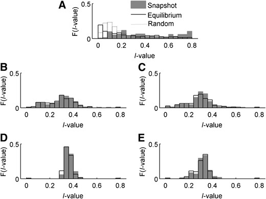
Frequency plots of I-values for all cases. Shaded area, snapshot results with five alleles; solid line, equilibrium results with five alleles. The dotted line in case 0 indicates the expected distribution of I-values for random allele frequencies. A–E represent cases 0–4 in order.
Case 0 had significant differences (P < 0.0001) between distributions of snapshot and equilibrium I-values, with equilibrium values shifted toward 0 due to the loss of rare transient alleles. Surprisingly, in cases 1–4 the systems with five alleles at snapshot or at equilibrium produce distributions of I-values that are not significantly different (two-sample Kolmogorov–Smirnov test, P = 0.72, 0.50, 0.25, and 0.59 for cases 1–4, respectively). Equally surprising are the shapes of those distributions. In cases 1–4, I-values show bell-shaped frequency distributions, centered above 0, that do not shift between snapshot and equilibrium. This suggests that these models produce polymorphisms that have skewed distributions (I > 0) and are also stable, being less likely to lose transient alleles on the way to equilibrium.
Analysis of fitness sets
Following Trotter and Spencer (2007), we divided the interaction-fitness values within each fitness set into nine fitness “classes”. Class divisions are set based on heterozygosity of, and allelic similarities between, the interacting genotypes. Subscripts denote homo- and heterozygosity, as well as allele sharing between interacting genotypes. Let the class of homozygote by unlike-homozygote interactions be Cii,jj, that of homozygote by like-homozygote interactions be Cii,ii, that of heterozygote by like-heterozygote interactions be Cij,ij, that of heterozygote by similar heterozygote interactions be Cij,jk, that of heterozygote by unrelated heterozygote interactions be Cij,kl, and so forth. For a given fitness set, each class value takes the mean of all interaction fitnesses in that class. The relative values of fitness class means can be taken to indicate different forms of frequency dependence. For example, we say fitness sets with low values of self–self interactions (Cii,ii and Cij,ij) exemplify negative frequency dependence, since low fitness in self-interactions causes lower relative fitness for common alleles.
In this analysis, we again focus on the case where n = 5. The cases n = 2, 3, and 4 of the PIM do not exhibit all fitness classes (again, see Trotter and Spencer 2007 for further discussion of this issue). For all cases, some snapshot fitness sets maintained all alleles at equilibrium from all initial conditions, some from only a few, and some from none at all. One might then expect to find some relationship between the contents of a snapshot fitness set and the size of the domain of attraction of its fully polymorphic equilibrium. For example, fitness sets with heterozygote advantage might keep all alleles more often than do fitness sets with homozygote advantage. In a parameter-space approach (Trotter and Spencer 2007), PIM fitness sets with low self-interaction fitnesses (Cii,ii, Cij,ij, Cij,jj, Cii,ij) had larger within-set potential for variation. We examined correlations between the proportion of initial conditions that maintain snapshot variation (P) and all C class values, using Spearman’s nonparametric ρ (rs). These relationships are summarized in Table 4. While all cases had significant correlations between P and at least one C, all such correlations are weak. Cases 1 and 2 have significant negative correlations between potential and the homozygote interaction classes (Cii,__) as well as the heterozygote self-self interaction class (Cij,ij). Cases 3 and 4 have significant positive correlations between P and most heterozygote fitness classes. Thus, cases 1 and 2 show some signal of negative frequency dependence, while cases 3 and 4 seem to show more effects of heterozygote advantage.
Correlations between C class values and potential to maintain snapshot variation at equilibrium
| Case 0 | Case 1 | Case 2 | Case 3 | Case 4 | ||||||
|---|---|---|---|---|---|---|---|---|---|---|
| Fitness class | rs | P | rs | P | rs | P | rs | P | rs | P |
| Cii,ii | −0.184* | 0.033 | −0.248** | 0.005 | −0.291** | 0.001 | 0.013 | 0.871 | −0.020 | 0.809 |
| Cii,jj | 0.044 | 0.615 | −0.005 | 0.955 | 0.109 | 0.214 | 0.033 | 0.688 | 0.015 | 0.861 |
| Cii,ij | 0.051 | 0.559 | −0.360** | 0.000028 | −0.110 | 0.211 | 0.035 | 0.666 | 0.039 | 0.641 |
| Cii,jk | 0.559 | 0.922 | −0.008 | 0.928 | 0.293** | 0.0006 | 0.004 | 0.961 | 0.064 | 0.442 |
| Cij,jj | −0.194* | 0.025 | −0.245** | 0.005 | −0.319** | 0.00019 | 0.023 | 0.774 | 0.186* | 0.024 |
| Cij,kk | −0.182* | 0.035 | −0.039 | 0.664 | −0.018 | 0.839 | 0.270** | 0.001 | 0.433** | 0.00000004 |
| Cij,ik | 0.063 | 0.469 | −0.076 | 0.391 | 0.037 | 0.676 | 0.117 | 0.149 | 0.283** | 0.001 |
| Cij,kl | −0.011 | 0.904 | 0.244** | 0.005 | 0.257** | 0.003 | 0.296** | 0.0002 | 0.436** | 0.0000003 |
| Cij,ij | 0.173* | 0.046 | −0.363** | 0.000023 | −0.200* | 0.021 | 0.054 | 0.508 | −0.042 | 0.617 |
Significant at the 0.05 level; **significant at the 0.01 level.
| Case 0 | Case 1 | Case 2 | Case 3 | Case 4 | ||||||
|---|---|---|---|---|---|---|---|---|---|---|
| Fitness class | rs | P | rs | P | rs | P | rs | P | rs | P |
| Cii,ii | −0.184* | 0.033 | −0.248** | 0.005 | −0.291** | 0.001 | 0.013 | 0.871 | −0.020 | 0.809 |
| Cii,jj | 0.044 | 0.615 | −0.005 | 0.955 | 0.109 | 0.214 | 0.033 | 0.688 | 0.015 | 0.861 |
| Cii,ij | 0.051 | 0.559 | −0.360** | 0.000028 | −0.110 | 0.211 | 0.035 | 0.666 | 0.039 | 0.641 |
| Cii,jk | 0.559 | 0.922 | −0.008 | 0.928 | 0.293** | 0.0006 | 0.004 | 0.961 | 0.064 | 0.442 |
| Cij,jj | −0.194* | 0.025 | −0.245** | 0.005 | −0.319** | 0.00019 | 0.023 | 0.774 | 0.186* | 0.024 |
| Cij,kk | −0.182* | 0.035 | −0.039 | 0.664 | −0.018 | 0.839 | 0.270** | 0.001 | 0.433** | 0.00000004 |
| Cij,ik | 0.063 | 0.469 | −0.076 | 0.391 | 0.037 | 0.676 | 0.117 | 0.149 | 0.283** | 0.001 |
| Cij,kl | −0.011 | 0.904 | 0.244** | 0.005 | 0.257** | 0.003 | 0.296** | 0.0002 | 0.436** | 0.0000003 |
| Cij,ij | 0.173* | 0.046 | −0.363** | 0.000023 | −0.200* | 0.021 | 0.054 | 0.508 | −0.042 | 0.617 |
Significant at the 0.05 level; **significant at the 0.01 level.
The patterns of fitness produced by cases 1 and 2 agree closely for all fitness classes (see Figures 6 and 7). Case 2 has mild heterozygote advantage built in, so it is surprising that its heterozygote fitnesses are not the highest. Strangely enough, the signal for heterozygote advantage itself is more clearly pronounced in the data from cases 3 and 4, where heterozygote class means are all higher than the corresponding homozygote class means (with the exception of the heterozygote self–self interaction, which is comparatively low in case 3). The trends produced by cases 1 and 2 are more indicative of negative FDS, where self-interaction fitnesses (interactions between genotypes with shared alleles) are minimal (see low values of Cii,ii, Cij,ij, and Cij,jj) with the exception of those with the least sharing and the most heterozygous, Cij,jk.
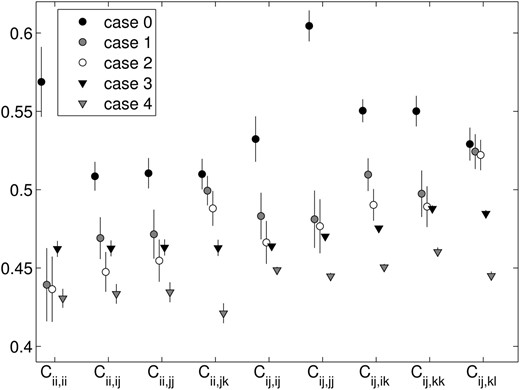
Snapshot fitness class means with 95% confidence intervals, from fitness sets with n = 5, from all five versions of the PIM construction approach.
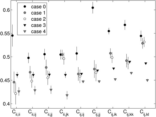
Equilibrium fitness class means with 95% confidence intervals, from fitness sets with n = 5, from all five versions of the PIM construction approach.
The fitness class means from the snapshot data (Figure 6) and in the equilibrium data (Figure 7) are similar, but with higher values in most classes at equilibrium, consistent with the loss of low-fitness transient alleles on the way to equilibrium.
Flavors of frequency dependence
To tease out common within-set patterns of fitness, we searched the fitness sets for commonly discussed selection regimes, using schemes listed in Table 5. To provide a basis for comparison, we also searched for these schemes in a sample of 105 “random” fitness sets, where each interaction fitness was drawn from the uniform distribution on [0, 1]. In the case of uniformly distributed fitness, negative FDS and positive FDS are equally probable. In the general construction model (case 0), we see that positive FDS is slightly more common (∼10% of sets) than negative FDS (∼7%) in snapshot, but that this relationship is reversed in the equilibrium sets (5% and 16%). In the simplest mutation-from-existing-alleles model (case 1), all of our defined flavors of FDS occur, with the exception of heterozygote disadvantage. Negative FDS is more common than positive FDS; and heterozygote advantage is more common than heterozygote disadvantage, which aligns with the usual intuitive understanding of how FDS should best maintain variation. In cases 1–4, negative FDS is always more common than in the sample of randomly generated fitness sets, and in cases 2–4 it is more common in equilibrium than in snapshot sets. Positive FDS occurs in all cases except case 3, but it is rare. Heterozygote advantage is very common in cases 3 and 4, but surprisingly not very common in case 2 (which has in-built heterozygote advantage). The addition of defined mutant impacts (cases 3 and 4) produces some notable changes. In case 3, negative FDS and heterozygote advantage are both present in ∼20% of fitness sets while in case 4, heterozygote advantage is common but negative FDS is strikingly rare.
Frequencies of selection schemes in model and random fitness sets
| Case 0 | Case 1 | Case 2 | Case 3 | Case 4 | Random: | |||||||
|---|---|---|---|---|---|---|---|---|---|---|---|---|
| Selection scheme | Definition | Snap | Equil | Snap | Equil | Snap | Equil | Snap | Equil | Snap | Equil | NA |
| Negative FDS | Cii,ii and Cij,ij < all others | 0.0746 | 0.157 | 0.124 | 0.123 | 0.106 | 0.117 | 0.216 | 0.2536 | 0.0544 | 0.0714 | 0.105 |
| Strict negative FDS | ↑shared alleles, ↓fitness: | |||||||||||
| Cii,ii,Cij,ij < Cii,ik, Cij,ik, Cij,jj < Cii,kk, Cii,kl, Cij,kk,Cij,kl | 0 | 0 | 0.0232 | 0.0351 | 0.0379 | 0.0541 | 0.0458 | 0.0580 | 0.0068 | 0.0102 | 0.0034 | |
| Positive FDS | Cii,ii and Cij,ij > all others | 0.097 | 0.0522 | 0.0543 | 0.0351 | 0.0227 | 0.009 | 0 | 0 | 0.0408 | 0 | 0.105 |
| Strict positive FDS | ↑shared alleles, ↑fitness: | |||||||||||
| Cii,ii,Cij,ij > Cii,ik, Cij,ik, Cij,jj > Cii,kk, Cii,kl, Cij,kk,Cij,kl | 0 | 0 | 0.0233 | 0.0088 | 0.0152 | 0.009 | 0 | 0 | 0.0204 | 0.0102 | 0.0034 | |
| Heterozygote advantage | Cij, > all Cii, __ | 0.0522 | 0.0696 | 0.0465 | 0.0175 | 0.0455 | 0.036 | 0.170 | 0.174 | 0.218 | 0.286 | 0.0087 |
| Homozygote advantage | Cij, < all Cii, __ | 0 | 0 | 0 | 0 | 0 | 0 | 0.0131 | 0.0073 | 0 | 0 | 0.0088 |
| Totals | All special cases above | 0.224 | 0.278 | 0.272 | 0.219 | 0.227 | 0.225 | 0.444 | 0.493 | 0.340 | 0.378 | 0.235 |
| N sets | 134 | 115 | 129 | 114 | 132 | 111 | 153 | 138 | 147 | 98 | 100,000 | |
| Value of 1 set | 0.007 | 0.009 | 0.008 | 0.009 | 0.0075 | 0.009 | 0.0065 | 0.007 | 0.007 | 0.01 | 0 | |
Snap, snapshot; Equil, equilibrium; NA, not applicable.
| Case 0 | Case 1 | Case 2 | Case 3 | Case 4 | Random: | |||||||
|---|---|---|---|---|---|---|---|---|---|---|---|---|
| Selection scheme | Definition | Snap | Equil | Snap | Equil | Snap | Equil | Snap | Equil | Snap | Equil | NA |
| Negative FDS | Cii,ii and Cij,ij < all others | 0.0746 | 0.157 | 0.124 | 0.123 | 0.106 | 0.117 | 0.216 | 0.2536 | 0.0544 | 0.0714 | 0.105 |
| Strict negative FDS | ↑shared alleles, ↓fitness: | |||||||||||
| Cii,ii,Cij,ij < Cii,ik, Cij,ik, Cij,jj < Cii,kk, Cii,kl, Cij,kk,Cij,kl | 0 | 0 | 0.0232 | 0.0351 | 0.0379 | 0.0541 | 0.0458 | 0.0580 | 0.0068 | 0.0102 | 0.0034 | |
| Positive FDS | Cii,ii and Cij,ij > all others | 0.097 | 0.0522 | 0.0543 | 0.0351 | 0.0227 | 0.009 | 0 | 0 | 0.0408 | 0 | 0.105 |
| Strict positive FDS | ↑shared alleles, ↑fitness: | |||||||||||
| Cii,ii,Cij,ij > Cii,ik, Cij,ik, Cij,jj > Cii,kk, Cii,kl, Cij,kk,Cij,kl | 0 | 0 | 0.0233 | 0.0088 | 0.0152 | 0.009 | 0 | 0 | 0.0204 | 0.0102 | 0.0034 | |
| Heterozygote advantage | Cij, > all Cii, __ | 0.0522 | 0.0696 | 0.0465 | 0.0175 | 0.0455 | 0.036 | 0.170 | 0.174 | 0.218 | 0.286 | 0.0087 |
| Homozygote advantage | Cij, < all Cii, __ | 0 | 0 | 0 | 0 | 0 | 0 | 0.0131 | 0.0073 | 0 | 0 | 0.0088 |
| Totals | All special cases above | 0.224 | 0.278 | 0.272 | 0.219 | 0.227 | 0.225 | 0.444 | 0.493 | 0.340 | 0.378 | 0.235 |
| N sets | 134 | 115 | 129 | 114 | 132 | 111 | 153 | 138 | 147 | 98 | 100,000 | |
| Value of 1 set | 0.007 | 0.009 | 0.008 | 0.009 | 0.0075 | 0.009 | 0.0065 | 0.007 | 0.007 | 0.01 | 0 | |
Snap, snapshot; Equil, equilibrium; NA, not applicable.
Discussion
In this series of simulations, we have investigated the effect of mutation from existing alleles on the potential for polymorphism under a construction approach to the PIM of FDS. We find that generating mutants from existing alleles lowers the average number of alleles found in a system subject to FDS under a construction approach, relative to previously studied models with uniformly distributed mutant fitnesses. Interestingly, while the overall numbers of alleles found at a given time point are lower, the polymorphisms produced are more stable, with more natural allele-frequency distributions.
Contrary to our intuitive expectation, the cases that were expected to produce more alleles actually had lower overall levels of polymorphism. The case with built-in heterozygote advantage (case 2) produced fewer alleles than the equivalent case with all mutant fitnesses drawn from the same distribution (case 1). The case in which mutant impacts are negative (case 4) produced fewer alleles than the case in which mutants are indistinguishable from their parent in terms of their impact on other alleles (case 3). This case, in which mutant impacts are strictly equal to parental impacts, produced the highest mean levels of polymorphism at both snapshot and equilibrium. This case is arguably the most biologically reasonable of the four, since mutants in case 3 are in general less fit than their parental allele, but have no or negligible effect on preexisting alleles. [It is generally accepted that the majority of new mutations are deleterious mutations of small effect, but there is no biological reason to expect that mutants should have deleterious impacts on other genotypes (as in case 4)]. Thus, it is interesting that case 3 produced the highest numbers of alleles.
The PIM is well known to generate decreases in mean fitness (Cockerham et al. 1972; Asmussen and Basnayake 1990; Asmussen et al. 2004; Trotter and Spencer 2007) and nonmonotonic mean-fitness trajectories (Trotter and Spencer 2009). However, if fitnesses are symmetric (or pseudosymmetric, see Matessi and Schneider 2009), the PIM does evolve to maximize mean fitness (or closely related quantities). Earlier construction approaches to the PIM found the mean fitness to be erratic and largely decoupled from the number of alleles (Trotter and Spencer 2008). In most of our simulations of cases 1–4, there were long periods of stable allele number and mean fitness, corresponding to particularly stable arrangements of fitness. However, given that the distributions of mutant fitnesses are functions of parental frequencies, it is always possible to produce a successful invader allele. No matter how fit or stable the current polymorphism is, there is no maximum mean fitness it could attain to cause permanent stability.
The most notable result in our measurements of mean fitness is the remarkable oscillations in mean fitness that occur regularly in both cases 1 and 2 and more rarely in cases 3 and 4. Interestingly, the dynamics of mean fitness and numbers of alleles appear to be independent during these oscillations. Several other studies have found complex dynamics produced by the PIM (Altenberg 1991; Gavrilets and Hastings 1995; Trotter and Spencer 2009) but only in systems where the number of alleles is fixed. While some definite patterns emerged from close investigation of the oscillations, no general rule applies to all cases. In general, sharp drops in mean fitness corresponded to multiple invasions of new alleles and sharp spikes in mean fitness occurred during multiple extinctions. In many cases, long periods of stability of allele numbers corresponded to monotonic decreases in mean fitness. These decreases in are most likely caused by the slow increase in frequency of an allele whose impact on other alleles is negative. The existence of mean fitness oscillations occurring entirely during periods of unchanging n is possibly related to replacement invasions or to the stable n undergoing allele-frequency cycles. The fact that increased ecological realism (i.e., mutation from existing alleles) in our approach to the PIM creates such counterintuitive mean-fitness trajectories suggests that non-hill-climbing evolution may have an important role in evolution when fitness is frequency dependent.
While it is clear that generating mutants from existing alleles increases the overall potential for stable polymorphism over the general construction approach to the PIM, there is no clear pattern in the potential for polymorphism among the mutation models. While many fitness sets (which we label “type I”) maintained all snapshot alleles from their snapshot allele-frequency vectors, the number of these fitness sets drops off dramatically as n increases. Similarly, regardless of the system used to generate new mutants, the models all evolve into areas of fitness space where heterozygotes are more fit than homozygotes. Strangely, however, the case with built-in heterozygote advantage in the mutations does not produce particularly high levels of polymorphism. Other recent studies (Marks and Ptak 2001; Star et al. 2007b; Stoffels and Spencer 2008; Trotter and Spencer 2008) agree that heterozygote advantage alone fails as an explanation for polymorphism when examined under constructionist approaches to a wide variety of selection models. Additionally, while our implementation of rare homozygous lethality in all cases does imply some very weak heterozygote advantage, in simulations without homozygous lethals (see File S1) we found that their omission had a negligible effect on numbers of alleles. Thus, while heterozygote advantage often emerges from the mutation–selection process, it does not seem to be key to producing large amounts of polymorphism.
Early parameter-space approaches suggested the conditions for multiple-allele polymorphisms are very restrictive (Trotter and Spencer 2007), whereas general construction approaches to the PIM easily generate very large numbers of alleles (Trotter and Spencer 2008). However, each addition of genetic realism (mutation from a parental allele and then the incorporation of negative mutant impacts) has decreased the level of polymorphism generated by the construction approach. Presumably the addition of drift to the models will further limit the level of polymorphism produced (investigations of such models are in progress). The level of polymorphism produced by construction approaches is, of course, sensitive to mutation rate (see File S1) but the rates of mutation used in our analyses here are consistent with those in the few empirical studies that are available (Drake et al. 1998). These results remind us that FDS alone, even strict negative FDS, is not a panacea for the paradox of polymorphism, and any attempts to explain large numbers of alleles as being due to FDS must be viewed with caution.
Acknowledgments
The authors thank Bastiaan Star and Rick Stoffels for helpful discussion and two anonymous reviewers for comments on the manuscript. This work was supported by the Marsden Fund of the Royal Society of New Zealand (contract U00315) and by the Allan Wilson Centre for Molecular Evolution and Ecology. M.V.T. was the recipient of a scholarship from the Division of Sciences of the University of Otago.
Footnotes
Communicating editor: L. M. Wahl
Literature Cited
Author notes
Supporting information is available online at http://www.genetics.org/lookup/suppl/doi:10.1534/genetics.113.152496/-/DC1.
