Estimating Selection Coefficients in Spatially Structured Populations from Time Series Data of Allele Frequencies

Abstract

DETECTING selection and estimating selection coefficients are important questions in many areas of genetics. In humans, genome-wide scans for selection identify regions of the genome that have been important in human evolution and provide clues about the location of important functional variants (Bustamante et al. 2005; Nielsen et al. 2005; Voight et al. 2006; Sabeti et al. 2007). In pathogen research, understanding selection can help to understand and control the evolution and spatial spread of drug resistance in both pathogens and vectors. In cancer, intra-tumor selection is an important driver of tumor growth and development (Bignell et al. 2010). With only a sample from one timepoint, for example, with the human selection scans described above, it is difficult to obtain quantitative estimates of selection coefficients. However, with time series data on allele frequencies, for example, from experimental evolution experiments, ecological observations, or ancient DNA, it is much easier (Bollback et al. 2008; Illingworth and Mustonen 2011; Malaspinas et al. 2012).

Most natural populations are structured and to separate out the effects of selection and demography, we need to take this into account. We focus on spatial structure since it is common and easily visualized. The spatial spread of a selected mutation is usually described using the traveling wave theory of Fisher (1937). This powerful tool can be extended to more complex situations such as the spread of multiple competing alleles (Ralph and Coop 2010) or the existence of spatially varying selection pressures (see Novembre and Di Rienzo 2009, box 1, for a brief review of such models). However these models can be difficult to fit to data. We analyze a lattice model of population subdivision, which can provide complex population structure, yet is simple enough that we can compute approximate maximum-likelihood estimates (MLEs) for the parameters.

Typically the analysis of time series data of allele frequencies uses a hidden Markov model (HMM) framework (Williamson and Slatkin 1999; Bollback et al. 2008). The allele frequency trajectory is modeled as a Markovian process, either a discrete process like the Wright–Fisher or Moran models or as a diffusion (i.e., the limiting case of the discrete models). The observations are modeled as binomial observations from this population. Williamson and Slatkin (1999) use this approach to compute a likelihood surface for the effective population size N_e, assuming no selection. A similar approach to estimating N_e is used by Anderson et al. (2000) and Wang (2001). To estimate the selection coefficient s, Bollback et al. (2008) use numerical techniques to compute a likelihood surface and estimate 2N_es. Malaspinas et al. (2012) use an approximate transition density to compute the likelihood. They do this for a grid of parameter values to estimate s and other parameters. Our method differs from these approaches in that we use an expectation-maximization (EM) algorithm to maximize the likelihood, rather than numerical search. We also show how to extend our approach to the estimation of spatially varying selection coefficients on a lattice, a problem that has not been considered before, but that is important in the study of naturally occurring populations.

Materials and Methods

In this section, we first describe the model and notation, and then derive the approximate MLEs for the parameters given complete observations of the allele frequency trajectory. Then we explain how to set up the HMM and how to solve it to obtain the MLE given incomplete observations. In each of these subsections we describe both the single population and the structured case.

Model

Single population:

Consider a haploid Wright–Fisher population of constant size 2N_e. We are interested in the frequency of a single allele with two types, A and a. Suppose the a allele has frequency f_t at generation t for t = 0, …, T. The a allele has selection coefficient s so the relative finesses of the A and a genotypes are 1 and 1 + s. Then at each generation t, the number of type a individuals is drawn from a binomial distribution with size 2N_e and probability $(1+s)ft−1/[1+sft−1]$⁠. We observe a sample of n_t individuals at generation t of which a_t are of the selected type, so that $at/nt$ is an empirical estimate of f_t. We can represent missing observations by setting n_t = 0. For sufficiently large 2N_e, and f_t not too small, we can approximate the distribution of the difference f_t+1 − f_t by a normal distribution with mean sf_t(1 − f_t) and variance $ft(1−ft)/2Ne$⁠.

To consider the effects of nonadditive selection, we consider a diploid population of size N_e (2N_e chromosomes). Assume that the three genotypes AA, Aa, and aa have relative fitnesses 1, 1 + 2hs, and 1 + 2s, respectively, where h is the heterozygous effect. The factor of 2 ensures that in the case of additive selection (⁠$h=12$⁠) the dynamics are the same as in the haploid case described above. h = 0 corresponds to a fully recessive allele and h = 1 to a fully dominant allele. In this case for large N_e we can approximate the distribution of the difference f_t+1 − f_t by a normal distribution with mean 2sf_t(1 − f_t)(f_t + h(1 − 2f_t)) and variance $ft(1−ft)/2Ne$⁠. See Ewens (1979) for a fuller discussion of this model.

Structured population:

For the structured population we consider a lattice model consisting of K² single populations each of size 2N_e, arranged in a K × K grid (Figure 1). Each deme has two, three, or four neighboring demes, depending on where it is located on the grid. At each generation, from each population, M individuals migrate to each neighboring deme. We also define the proportional migration rate $m=M/2Ne$⁠. We index the demes by i, j ε {1, … K} and write κ_ij for the set of indices of demes that neighbor deme i, j. The frequency of the selected allele in population i, j at generation t is $ftij$⁠. The migration rate is constant over all demes and time. The selection coefficients are constant over time, but not necessarily across demes. We write s^ij for the selection coefficient in deme i, j. We also write $ntij$ for the size of the sample taken from deme i, j at generation t and $atij$ for the number of that sample of the selected type.

Figure 1

Open in new tabDownload slide

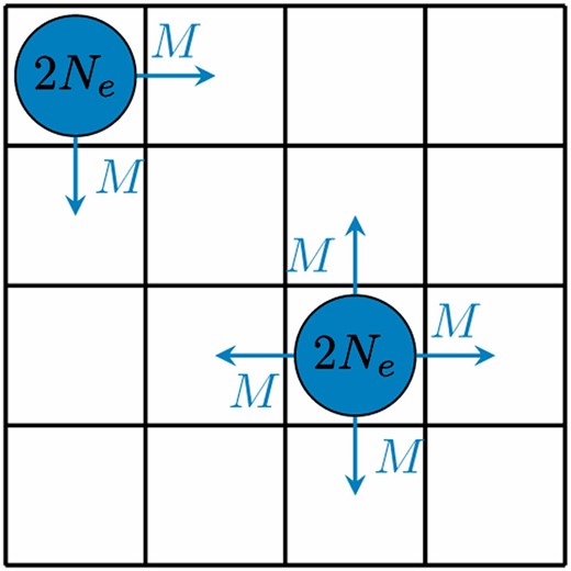
The Wright–Fisher lattice model, shown for K = 4. Each deme has a constant population size of 2N_e and in each generation, exactly M individuals migrate to each of the neighboring demes.

Maximum-likelihood estimators

Single population:

Structured population:

In the structured case, we would like an expression for the joint MLE of m and the s^ij. This does not have a simple form, but by considering a slightly simplified process we can obtain an expression for the MLE’s of s^ij and m, similar to those derived for single populations.

Estimation using hidden Markov models

Single population:

To apply standard HMM theory, we discretize the allele frequency space, assuming that f_t ε = {g₀, … g_D}, and the interval between points δg = g_i+1 − g_i is constant for all i. We typically use a grid size of D = 100. We define the HMM as follows:

1. The hidden states are the frequencies f_t. The observations are the number of alleles of the selected type a_t. The parameters N_e and n_t are known, and we have an estimate of s, which we take as fixed for this iteration.

2. The emission probabilities are binomial: a_t ∼ Bin(n_t, f_t).

3. The transition probabilities are defined by integrating the approximate normal continuous transition density between the midpoints of the intervals of the discretized points:

   $P{ft+1=g|ft}=∫g−δg/2g+δg/2φ(x−μtσt)dx,$

   (16)

where

$μt=ft+sft(1−ft)andσt2=ft(1−ft)2Ne.$

(17)

We can proceed in several ways from here. Given a value of s, we can compute the likelihood of the observations, so we could just find the value of s that maximizes this likelihood, either by searching or by standard numerical maximization techniques. However, this would become impractical in the structured case, and a more efficient way to find the MLE is with an EM algorithm, where, at each iteration, we update the estimate of s using the value that maximizes the expected log-likelihood under the posterior distribution on the hidden variables f_t, conditional on the previous estimate of s. Supose at iteration r, we have an estimate s_r of s; then taking the expectation of Equation 2, expanding to first order in s, and maximizing yields the EM update rule for the next estimate of s, analogous to Equation 4,

$sr+1=E[fT]−E[f0]Σt=0T−1E[ft(1−ft)],$

(18)

where the expectations are taken with respect to the posterior distribution of paths, conditional on the observations, and the selection coefficient s_r. These posterior probabilities can be computed using the forward–backward algorithm. This expression is identical to Equation 4 but with expectations replacing the actual frequencies. Taking into account the discretization of the frequencies, our algorithm is as follows:

1. Initialization: Choose s₀ to be some reasonable starting value. We linearly interpolate the frequency estimates and apply Equation 4.

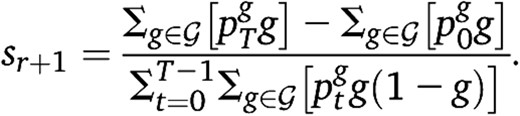
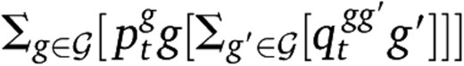
2. Recursion: Given an estimate s_r for s, apply the forward–backward algorithm to the HMM described above to compute the probabilities $ptg=P{ft=g|a0,…,aT,sr}$⁠. Then set

3. Termination: Stop when |s_r+1 − s_r| < ε for some predetermined tolerance ε and set our estimate of s equal to s_r+1.

(19)

Open in new tabDownload slide

The algorithm also naturally computes (as part of the forward algorithm) the likelihood of the data at each iteration given the observations and the current parameter values. Using the final likelihood, and the fact that the difference in likelihood between two models is asymptotically χ² distributed, we can compute confidence intervals and P-values against various null hypotheses for our estimates.

If the dominance parameter h ≠ 0.5, then the update rule in Equation 18 becomes

$sr+1=Σt=0T−1E[ht(ft+1−ft)]2Σt=0T−1E[ht2ft(1−ft)],$

(20)

where h_t = f_t + h(1 − 2f_t). Since h_t depends on f_t, the numerator now contains a $E$[f_t+1f_t] term that makes this expression harder than Equation 19 to compute in the discretized model. Fortunately, using the forward and backward probabilities, it is possible to compute the conditional transition probabilities $qtgg′=P{ft+1=g′|ft=g,a0,…,aT,sr}$ and using these, we compute $E$[f_t+1f_t] in the discretized step using . Equation 19 is then replaced by

(21)

Open in new tabDownload slide

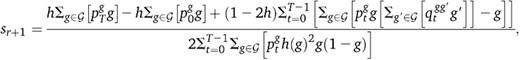
where h(g) = g + h(1 − 2g).

Structured population:

Directly extending the EM algorithm to the structured case is difficult for two reasons. First, the likelihood depends on both the s^ij and m, making the EM step difficult to calculate. Second, the state space of the HMM increases rapidly with the number of demes. If there are K² demes and D discretized states, then the full HMM has $DK2$ states, making it impractical to compute for anything but the smallest number of demes. Therefore, we present an algorithm that makes two approximations to make the solution tractable. First, we update s^ij and m separately. The update rule for s^ij has the form of the EM update rule from the single population case and the update rule for m can be computed similarly. Second, when updating any frequency in any particular deme, we assume that the allele frequencies in all the other demes are fixed to their most likely values from the previous iteration, which makes the HMM calculations independent across demes, reducing the complexity to DK².

1. Initialization: Compute an initial guess for the $ftij$⁠, by taking the observed frequencies and linearly interpolating missing values. Call this $f˜tij$ and make initial guesses for s^ij and m.

2. Recursion: Given estimates $srij$⁠, $mr$ and $f˜tij$ for $sij$⁠, m and $ftij$⁠, solve the HMM for each deme as in the single population case. Compute the posterior probabilities $pij,tg=P{ftij=g|a0ij…atij,sij}$ as before, and the most likely path $vtij$⁠, using the Viterbi algorithm. Compute new estimates $sr+1ij$ and m_r+1 using the EM update rules above, and set $f˜t+1ij=vtij$⁠.

3. Termination: Stop when the change in log-likelihood between successive iterations is less than some specified amount ε.

Note that the calculation for each of the K² demes is independent, so it would be easy to parallelize this computation and compute the recursion step for each deme on a separate core.

Data sets

To test our algorithms, we simulated data from both the single and structured Wright–Fisher models described above and checked whether we could recover the parameters used to simulate. We investigated the behavior of our algorithms for a range of parameter values (see Results). To test the algorithm on real data, we turned to classical data sets of morph frequencies in two moth species. These data sets are described below.

Single population:

For a data set of allele frequencies in a single, closed population, we used observations of frequencies of the medionigra morph in a population of Panaxia dominula (scarlet tiger moth) at Cothill Fen near Oxford. Observations of this colony were first made in 1939 by E. B. Ford and R. A. Fisher and were collected annually, with some gaps, until at least 1999. The data are reported in Cook and Jones (1996) and Jones (2000) and have most recently been analyzed by O’Hara (2005). P. dominula is a colorful day-flying moth, which has exactly one generation per calendar year. The medionigra morph is the result of a heterozygous polymorphism and is observed as a reduction of the size and number of white spots on the moths wings (see Fisher and Ford 1947 for a photograph of the various morphs). A moth that is homozygous for the variant allele is much darker, but this bimacula morph is much rarer and almost never observed. When the study was started, the medionigra morph was present in the Cothill colony at a frequency of ∼10%, but subsequently dropped sharply. The question of whether this rapid decline in frequency represented the effect of natural selection was the subject of a spirited debate between Fisher and S. Wright (Fisher and Ford 1947; Wright 1948). In our analysis, we assumed that the frequency of the medionigra morph corresponded exactly with the frequency of the allele. We also made the assumption that the effective population size is constant. As part of the collection of moth frequencies, the population size has been estimated using capture–recapture methods. Estimates have ranged from 216 to 60,000. Even if the census population really took this range, it is not clear what relation this has to the effective population size. We therefore assumed that the effective population size, 2N_e was constant, but checked whether different values of N_e had an effect on our results.

Structured population:

For our structured population data set, we turned to another classical data set on moth morph frequencies, this one of the species Biston betularia (peppered moth). The morph of interest here is the carbonaria morph, which appears very dark or black, in contrast to the typica morph, which has a complex speckled pattern on a light background. A full discussion of the extensive literature on this species is beyond the scope of this article (but see Cook 2003 for a review). Briefly, the carbonaria morph was identified in the north of England by 1848 and by 1958 was present at a frequency of ∼100% in the northwest, and at varying frequencies throughout the rest of the country (Kettlewell 1958). Starting in the early 1970s, the frequency of the carbonaria morph began to decline until today it is found very rarely. The change in frequency of the morph is almost certainly the result of a strong selective pressure, initially positive and changing direction some time in the mid 20th century. The exact nature of the selective pressure is still debated, but is generally considered to be related to industrial pollution caused by the burning of coal. There is also an intermediate form, insularia, controlled by different alleles at the same locus (Lees and Creed 1977). It is relatively rare (<10% of observations), and we excluded it from our analysis.

We searched the literature for observations of the frequency of the carbonaria morph across England since 1958 (we were able to extract data from 8 of these 12 references: Kettlewell 1958; Lees and Creed 1975; Bishop et al. 1978; Mani and Majerus 1993; West 1993; Clarke et al. 1994; Grant et al. 1996, 1998; Cook et al. 1999, 2002, 2005; Cook and Turner 2008; supporting information, File S1). Many data points had been reported more than once, and we attempted to remove duplicate observations. For each observation we extracted the number of moths collected, the numbers of typica and carbonaria observed, and the location of the observation. Assuming a single dominant allele and Hardy–Weinberg equilibrium, we converted the carbonaria frequency to an allele frequency as $f=1−1−fc$⁠, where f_c is the carbonaria frequency. We then assigned the observations to large UK Ordnance Survey grid squares. One of the corner grid squares lies entirely in the North Sea and had no observations. We filled this in by averaging over the two adjacent squares, reasoning that this would have the least disruption on the dynamics of the rest of the grid.

Results

Simulated data

Single population:

We simulated observations from single populations using the model described above. For each simulation, given a fixed population size and selection coefficient, we sampled allele frequencies at each generation using the binomial sampling probabilities in Equation 1. Then, given these frequency trajectories, we simulated samples of fixed sizes at known timepoints, by drawing a sample of fixed size, with replacement, with probability equal to the sample allele frequency.

First (Figure 2A) we investigated the effect of changing the sample size while the frequency of sampling remained constant. As expected, the error decreases with sample size, although for all effective population sizes, the expected error remains more or less constant above a given sample size. This constant error is larger when the effective population size is smaller. In Figure 2B, we show the effect of changing the frequency of sampling, ranging from sampling just the start and end points, to sampling at every generation, while keeping the sample size fixed. We see that the error decreases as the sampling frequency increases, but this really makes a difference only when the effective population size is small. For 2N_e = 10⁴, for example, changing the sampling frequency from every 20 generations to every generation makes virtually no difference to the error. One caveat is that this result relies on the start and end points being at some intermediate (between 0 and 1) frequency. If all we observed was that f₀ = 0 and f_T = 1 for some T, then it would be impossible to make a sensible estimate of s. We can see this further by varying the initial frequency (Figure 2C). Conditional on eventual fixation, the error increases as the initial frequency increases, demonstrating that it is the observations at intermediate allele frequencies that give us precision in our estimates. Again, this is particularly true when the effective population size is small.

Figure 2

Open in new tabDownload slide

Performance of the single population estimator. (A–D) Median absolute error of estimates of s, for a range of different parameter values. In each case, results are shown for effective population sizes 2N_e = 10², 10³ and 10⁴. Simulations were performed in a standard Wright-Fisher model and each point is the median of 100 independent simulations. If not otherwise specified, parameters are constant as follows: initial frequency f₀ = 0.5, number of generations T = 100, selection coefficient s = 0.05, samples taken every 10 generations, size of each sample = 100. We stopped the algorithm when successive estimates of s differed by less that ε = 10⁻³. (A) The size of the sample varies from 1 to 1000. (B) The frequency of sampling varies from 0.01 (once every 100 generations, i.e., two observations), to 1 (every generation). (C) The initial frequency f₀ varies from 0.1 to 0.9. (D) The selection coefficient s varies from 0 to 0.1. Inset: density of $s^$ for s = 0.1.

We also investigated the effect that s has on the error (Figure 2D). As s increases, the expected error increases, for all population sizes, although the relative error is decreasing. For large N_e and large s, the estimator begins to perform poorly beacause although the variance of $s^$ decreases, the bias increases (Figure 2D inset). The bias comes from the fact that our estimator is accurate only to O(s²).

Overall, it seems that the main determinant of the accuracy of the estimator is the effective population size of the underlying population and that, provided we have a sufficiently large population and at least some observations at intermediate allele frequencies, we require neither large nor frequent samples.

Finally, we checked whether the discretization and approximate transition density had a large influence on the result. In the single population model, if we set D = 2N_e + 1 and use the exact binomial transition probabilities (Equation 1) in the HMM rather than the approximate normal transition probabilities in Equation 17, then our model is exactly the one from which we simulated. We compared the estimates from this exact model to those from our approximate model. Using the same parameters as in Figure 2D, we found that the error increased with s, although modestly. When s = 0 the expected error in s due to discretization was ≈3 × 10⁻⁵ and when s = 0.1 the expected error was ≈3 × 10⁻³.

Structured population:

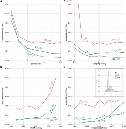
We simulated trajectories under the structured Wright–Fisher model, with selection coefficients varying across space and investigated the distribution of our estimates. We find that, as in the one-dimensional case, the estimates are more accurate the more of the trajectory we see. When we set f₀ = 0.5 so that each deme saw roughly the same change in trajectory, we found that our estimates for both s and m were unbiased (Figure 3A), but that when we set f₀ to 0.1, so that we saw less of the trajectory in demes with lower selection coefficients, we found that our estimates of the low selection coefficients were significantly worse (Figure 3B), consistent with what we would expect from the results in Figure 2C. We assumed that we could guess an initial value for m within 0.01 of the true value. If we set the initial value for m much further from the true value, then the estimator performed poorly.

Figure 3

Open in new tabDownload slide

Performance of the structured population estimator. We simulated observations from the structured Wright–Fisher model described in the main text, with 16 demes. Here 2N_e = 1000, s ranges across space from −0.06 to +0.06, m ranges from 0 to 0.1, samples of size 100 are taken every 10 generations. The algorithm is terminated when successive log-likelihoods differ by <0.1. The initial value for m is uniformly distributed on [m − 0.01, m + 0.01]. (A) Density plots of the results of 100 simulations, with m = 0.04 and f₀ = 0.5. Solid vertical lines show the true values, and dashed lines the mean of the density Top: Density of estimates of s. We combined the results across all demes with the same values of s, so the dark green density shows the results for 400 observations, i.e., 4 demes in each of 100 simulations. The inset shows the spatial distribution of selection coefficients, and an example path. Bottom: Density of estimates of m. (B) As A except f₀ = 0.1 and m = 0.05. (C and D) Median absolute error of the estimates of s in each deme, with different lines for each true value of s, for different values of m. f₀ = 0.1. (C) Error when m is unknown (but guessed to within 0.01), including error in m. (D) Error in s when m is known and fixed.

We investigated the performance of the estimator for different values of m (Figures 3, C and D). As m increased, the error in our estimates of s and m increased. We also investigated the error in our estimates of s when m was known and fixed (Figure 3D). In this case, there is a modest improvement in accuracy, particularly for small m (comparing Figures 3, C and D).

Real data

Single population:

The P. dominula data are shown in Figure 4, along with the likelihood surface for the true allele frequency trajectory and the likelihood function for s. We stopped the algorithm when successive iterations of s differed by <10⁻³. Taking 2N_e = 1000, we estimate a selection coefficient of −0.057, although with a fairly wide 95% confidence interval of (−0.113, −0.003). We thus reject the null hypothesis that s = 0 at the 5% level, but only just (twice the change in log-likelihood, 2Δℓ = 4.2, approximate $χ12$P-value = 0.04) and more or less agree with the original conclusion of Fisher and Ford (1947) that “the observed fluctuations in gene frequency are much greater than could be ascribed to random survival only.” Our estimate is similar to the estimate given by Cook and Jones (1996) and is consistent with results from other P. dominula colonies given in the same source. Wright (1948) argued that 2N_e might be of the order of 100 and O’Hara (2005) estimated it to be of the order of a few hundred. If 2N_e = 100, we would not reject s = 0 (2Δℓ = 0.45, approximate $χ12$P-value = 0.50). A recessive model fits with a higher likelihood, (change in log-likelihood, Δℓ = +2.5 for h = 0 compared to $h=12$⁠), but fits a large negative selection coefficient $s^≈−1$⁠, which is outside the range for which our approximations are valid, but may indicate that a model of recessive lethality (or near lethality) is the best explanation for the data.

Figure 4

Open in new tabDownload slide

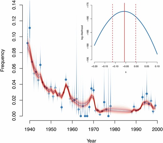
Panaxia dominula data. Main plot: medionigra frequency across generations. Blue dots show observed points with shaded support intervals. Red lines show posterior confidence intervals for the true frequency, from 10% (darkest) to 90% (lightest). Inset: log-likelihood as a function of s. For each value of s, we computed the likelihood of the observations using the forward algorithm for HMMs. Red solid and dashed lines show the MLE and the 95% confidence interval respectively. This figure shows the results for a model of additive selection although, as discussed in the main text, a recessive model may fit better.

Structured population:

To analyze the B. betularia data, we used m = 0 as an initial value and stopped when successive log-likelihoods differed by <0.005. If we assume that 2N_e = 1000, we estimate selection coefficients for the carbonaria allele varying spatially between 0 and −0.12. We also estimate that $m^=0.00$⁠. If we constrain s to be constant across the range, we estimate that $s^=−0.068$⁠; however, we strongly reject the hypothesis that s is constant (2Δℓ = 67, approximate $χ152$P-value = 1.7 × 10⁻⁸). Cook (2003) gives estimates for s from different sites ranging from −0.018 to −0.208. There are three data points, all consisting of observations from Kettlewell (1958), which have a large influence on the result that selection is not constant. If these are removed, then the P-value is less significant (2Δℓ = 36, approximate $χ152$P-value = 1.9 × 10⁻³). The model of dominant selection fitted better than additive or recessive selection (Δℓ = −36 and +10 for h = 0 and h = 1 compared to $h=12$⁠). The fit of the dominant model is shown in Figure 5. In this case we reject the hypothesis of constant selection even more strongly (2Δℓ = 111, approximate $χ152$P-value = 9.6 × 10⁻¹⁷).

Figure 5

Open in new tabDownload slide

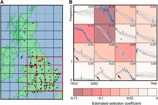
Biston betularia data. (A) Sample sites. The gray grid shows UK Ordnance Survey national grid reference squares. The red highlighted squares indicate the range we considered for our analysis. Black dots indicate sample sites. Red triangles indicate sites with observations in five or more years. We excluded sites outside the red area. (B) Estimated selection coefficients for the carbonaria allele. Each grid square represents a single deme. Time in generations runs along the x-axis in each deme from 1953 to 2002. Allele frequency runs on the y-axis in each deme from 0 to 1. Blue dots are observations, collapsed over all sites in a deme for each year. Gray lines are sample paths from the final pseudoposterior distribution. The background color of each deme represents the MLEs of the selection coefficients, which are given in the top right corner of each deme. We assumed 2N_e = 1000 (in each deme) and complete dominance (h = 1). Arrows indicate points of high influence (all from Kettlewell 1958). If these points are removed then the $s^ij$ in these demes lies between −0.12 and −0.10. The northwest and southeast squares each have observations in only 1 year, so the likelihood is almost completely flat.

Discussion

We developed an HMM-based maximum-likelihood estimator for selection coefficients in a panmictic population. Although this estimator cannot practically be extended to the structured case, we presented an approximate algorithm inspired by it that can estimate selection coefficients, migration rates, and allele frequencies in the Wright–Fisher lattice model. There are many effects, such as time- or state-varying parameters, that we do not include. A model incorporating all of these effects would probably be ill specified. However, any one of these effects could individually be incorporated into the model without much difficulty, to test specific hypotheses. For example, to test whether selection was constant across space, we used the estimator in Equation 13 rather than that in Equation 11 in our algorithm and compared the likelihoods.

Although our structured estimator is not a maximum-likelihood estimator, it has the property that it reduces to the one-dimentional estimator in the case where the migration rate is zero, or there is only a single deme. It is difficult to say much in general about the behavior of the estimator, other than we expect that its performance will worsen as m increases. Simulations supported this view, although the performance was still acceptable even for relatively large values of m (Figure 3, C and D).

To demonstrate these methods, we analyzed data about two British moth species. First, in an unstructured population, we investigated the evidence for selection on the medionigra allele in the Cothill P. dominula colony. We find that our conclusion depends largely on the assumptions that we make about effective population size, which is essentially the conclusion we reach by reading Fisher and Ford (1947) and Wright (1948). It is not surprising, given the form of our estimator, that the past 50 years of observations when f is very small do not add much to this estimate. However, the fact that the allele was still present after 60 years does give more support to the idea of a selection on recessive phenotype. Simulating under a Wright–Fisher model of diploid selection using f₀ = 0.1, we find that under a fully recessive lethal model, ∼58% of trajectories have not fixed at 0 by T = 60, compared to 41% under our best-fit additive model.

When we analyzed the B. betularia data, we found strong evidence that selection was not constant across the range, a conclusion that is robust to the assumptions we make about population size. However, it seems likely that several of our assumptions are violated in this population. In particular, given the rapid increase in carbonaria frequencies in the first half of the 20th century followed by the rapid decrease observed since, it seems likely that the sign of s switched from positive to negative at some point, making our assumption of time-constant s since 1953 implausible. The highly significant P-values we obtained are likely due, at least in part, to poor model fit. To incorporate time-varying selection into this model, we could include an additional HMM step to fit s as a function of t, subject to some assumptions about the rate of change of s. Model comparisons indicated that selection was dominant, which is consistant with the fact that the allele is dominant for the carbonaria trait (although note that this does not imply that selection must act dominantly, since the allele may have pleiotropic effects).

Our estimator generally converges rapidly. In the single population case, we found that the difference between s_r and the final estimate of s was roughly proportional to somewhere between $r−12$ and r⁻¹, depending on the observations. In practice, all our simulations converged within five iterations, and our P. dominula data converged after three. Convergence in the structured case was slower, particularly when m was unknown. Our B. betularia data took 17 iterations to converge. It would be easy to run each deme in parallel, although we have not implemented this. If we did, then each iteration of the structured case would take roughly the same time as the unstructured case, although it would still take more iterations to converge.

Finally we consider other data sets for which our methods could provide useful analysis. Ecological data sets about the spatial spread of alleles are the most obvious example, for example, data about the spread of drug resistance alleles in pathogens or vectors. Another interesting area, where data are just starting to become available, is the analysis of ancient DNA to learn about the recent evolution of humans and other species. In principle, relatively little data would be required to make inference in this setting, the critical requirement being that sampling density is sufficient to observe the frequency trajectory at intermediate values. Finally we note that our methods are very general in scope and could be applied not only to genetic data, but to the spread of any variation in space. We could use exactly the same techniques to analyze the spread of invasive species in a new ecosystem or the spread of cultural variation in a population.

Acknowledgments

We thank two anonymous reviewers whose comments greatly improved the manuscript. This work was supported by the Wellcome Trust (Grants [089250/Z/09/Z] to I.M. and [090532/Z/09/Z] to the Wellcome Trust Centre for Human Genetics).

Literature Cited

Footnotes

Author notes