


Abstract
Current efforts in systems genetics have focused on the development of statistical approaches that aim to disentangle causal relationships among molecular phenotypes in segregating populations. Reverse engineering of transcriptional networks plays a key role in the understanding of gene regulation. However, transcriptional regulation is only one possible mechanism, as methylation, phosphorylation, direct protein–protein interaction, transcription factor binding, etc., can also contribute to gene regulation. These additional modes of regulation can be interpreted as unobserved variables in the transcriptional gene network and can potentially affect its reconstruction accuracy. We develop tests of causal direction for a pair of phenotypes that may be embedded in a more complicated but unobserved network by extending Vuong’s selection tests for misspecified models. Our tests provide a significance level, which is unavailable for the widely used AIC and BIC criteria. We evaluate the performance of our tests against the AIC, BIC, and a recently published causality inference test in simulation studies. We compare the precision of causal calls using biologically validated causal relationships extracted from a database of 247 knockout experiments in yeast. Our model selection tests are more precise, showing greatly reduced false-positive rates compared to the alternative approaches. In practice, this is a useful feature since follow-up studies tend to be time consuming and expensive and, hence, it is important for the experimentalist to have causal predictions with low false-positive rates.
A key objective of biomedical research is to unravel the biochemical mechanisms underlying complex disease traits. Integration of genetic information with genomic, proteomic, and metabolomic data has been used to infer causal relationships among phenotypes (Schadt et al. 2005; Li et al. 2006; Kulp and Jagalur 2006; Chen et al. 2007; Zhu et al. 2004, 2007, 2008; Aten et al. 2008; Liu et al. 2008; Chaibub Neto et al. 2008, 2009; Winrow et al. 2009; Millstein et al. 2009). Current approaches for causal inference in systems genetics can be classified into whole network scoring methods (Zhu et al. 2004, 2007, 2008; Li et al. 2006; Liu et al. 2008; Chaibub Neto et al. 2008, 2010; Winrow et al. 2009; Hageman et al. 2011) or pairwise methods, which focus on the inference of causal relationships among pairs of phenotypes (Schadt et al. 2005; Li et al. 2006; Kulp and Jagalur 2006; Chen et al. 2007; Aten et al. 2008; Millstein et al. 2009; Li et al. 2010; Duarte and Zeng 2011). In this article we develop a pairwise approach for causal inference among pairs of phenotypes.
Two key assumptions for causal inference in systems genetics are genetic variation preceding phenotypic variation and Mendelian randomization of alleles in unlinked loci. These conditions together, which provide temporal order and eliminate confounding of other factors, justify causal claims between QTL and phenotypes. Causal inference among phenotypes is justified by conditional independence relations under Markov properties (Li et al. 2006; Chaibub Neto et al. 2010).
Given a pair of phenotypes, Y1 and Y2, that co-map to the same quantitative trait locus, Q, our objective is to learn which of the four distinct models, M1, M2, M3, and M4, depicted in Figure 1, is the best representation for the true relation between Y1 and Y2. Models M1, M2, M3, and M4 represent, respectively, the causal, reactive, independence, and full models as collapsed versions of more complex regulatory networks. For instance, when the data are transcriptional and one gene is upstream of other genes, the regulation of the upstream gene may affect those downstream, even when the regulation takes place via post-transcriptional mechanisms and, hence, is mediated by unobserved variables. Transcriptional networks should be interpreted as collapsed versions of more complicated networks, where the presence of an arrow from a QTL to a phenotype or from one phenotype to another simply means that there is a directional influence of one node on another (that is, there is at least one path in the network where the node in the tail of the arrow is upstream of the node in the head). Supporting Information, Figure S1 shows a few examples of networks and their collapsed versions. Our goal in this article is to infer the causal direction between two nodes, and the term “causal” should be interpreted as causal direction, meaning either direct or indirect causal relations.
In this article, we propose novel causal model selection hypothesis tests and compare their performance to the AIC and BIC model selection criteria and to a causality inference test (CIT) proposed by Millstein et al. (2009). AIC (Akaike 1974) and BIC (Schwarz 1978) are widely used penalized likelihood criteria performing model selection among models of different sizes. Overparameterized models tend to overfit the data and, when comparing models with different dimension, it is necessary to counterbalance model fit and model parsimony by adding a penalty term that depends on the number of parameters. CIT is an intersection-union test, in which a number of equivalence and conditional F tests are conservatively combined in a single test. P-values are computed for models M1 and M2 in Figure 1, but not for the M3 or M4 models, and the decision rule for model calling goes as follows: (1) call M1 if the M1 P-value is less than a significance threshold α and the M2 P-value is greater than α; (2) call M2 if it is the other way around; (3) call Mi if both P-values are greater than α; and (4) make a “no call” if both P-values are less than α. The Mi call actually means that the model is not M1 or M2 and could correspond to an M3 or M4 model. Note that the CIT makes a no call when both M1 and M2 models are simultaneously significant.
Our causal model selection tests (CMSTs) adapt and extend Vuong’s (1989) and Clarke’s (2007) tests to the comparison of four models. Vuong’s model selection test is a formal parametric hypothesis test devised to quantify the uncertainty associated with a model selection criterion, comparing two models based on their (penalized) likelihood scores. It uses the (penalized) log-likelihood ratio scaled by its standard error as a test statistic and tests the null hypothesis that both models are equally close to the true data generating process. While the (penalized) log-likelihood scores can determine only whether, for example, model A fits the data better than model B, Vuong’s test goes one step further and attaches a P-value to the scaled contrast of (penalized) log-likelihood scores. In this way it can interrogate whether the better fit of model A compared to model B is statistically significant. Vuong’s test tends to be conservative and low powered. Clarke (2007) proposed a nonparametric version that achieves an increase in power at the expense of higher miss-calling error rates by using the median rather than the mean of (penalized) log-likelihood ratio.
We propose three distinct versions of causal model selection tests: (1) the parametric CMST test, which corresponds to an intersection-union test of six separate Vuong’s tests; (2) the nonparametric CMST test, constructed as an intersection-union test of six of Clarke’s tests; and (3) the joint-parametric CMST test, which mimics an intersection-union test and is derived from the joint distribution of Vuong’s test statistics. These CMST tests inherit from Vuong’s test the property that none of the models being compared need be correct. That is, the true model may describe a more complicated network, including unobserved factors. Our approach simply selects the wrong model that is closest to the (unknown) true model.
Methods
Vuong’s model selection test
The Kullback–Leibler Information Criterion (KLIC) (Kullback 1959) measures the closeness of a probability model to the true distribution of data. Sawa (1978) showed that the KLIC orders approximate models by comparing the expected value of the log likelihood under the true model. Vuong (1989) used this result to develop an empirical test of two models based on the sample mean of the log-likelihood ratio scaled by its sample standard error.
The P-value of Vuong’s test is given by p12 = P(Z12 ≥ z12) = 1 − Φ(z12), where Φ() represents the cumulative density function of a standard normal variable (Vuong 1989). Note that since Z12 = −Z12; p21 = 1 − Φ(z21) = Φ(z12), so that p12 + p21 = 1. This property of the Vuong’s test ensures that the P-values of the intersection-union tests cannot be simultaneously significant.
Figure S2 illustrates how Vuong’s test trades a reduction in false positives against a reduction in statistical power. In our applications we need to account for both nested and nonnested models. While the presented test corresponds to Vuong’s test for strictly nonnested models, it is also valid for nested models when we adopt penalized likelihood scores (see File S1, for further details).
Clarke’s model selection paired sign test
Causal model selection tests
The four models M1, M2, M3, and M4 (Figure 1) are used to derive intersection-union tests based on the application of six separate Vuong (or Clarke) tests comparing, namely, f1 × f2, f1 × f3, f1 × f4, f2 × f3, f2 × f4, and f3 × f4. Sun et al. (2007) implicitly used intersection unions of Vuong’s tests to select among three nonnested models. Here, we present three distinct versions of the CMST: (1) parametric, (2) nonparametric, and (3) joint-parametric CMST tests. We implement the tests with penalized log likelihoods, but state results for log likelihoods.
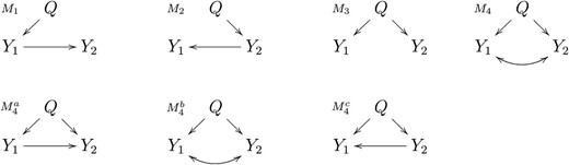
Pairwise causal models. Y1 and Y2 represent phenotypes that co-map to the same QTL, Q. Models M1, M2, M3, and M4 represent, respectively, the causal, reactive, independent, and full model. In model M1 the phenotype Y1 has a causal effect on Y2. In M2, the phenotype Y1 is actually reacting to a causal effect of Y2, hence the name reactive model. In the independence model, M3, there is no causal relationship between Y1 and Y2 and their correlation is solely due to Q. The full model, M4, corresponds to three distribution equivalent models , , and which cannot be distinguished as their maximized-likelihood scores are identical. Model represents a causal independence relationship where the correlation between Y1 and Y2 is a consequence of latent causal phenotypes, common causal QTL, or of common environmental effects. Models and correspond to causal-pleiotropic and reactive-pleiotropic relationships, respectively.
The nonparametric CMST test corresponds to an intersection union of Clarke’s tests, exactly analogous to the parametric version. Because in practice p12 + p21 ≈ 1 for Clarke’s test, the nonparametric CMST test also does not allow the detection of more than one significant model P-value.
Model selection tests for models M1, M2, M3, and M4
| H0 | Null distribution | P-value |
|---|---|---|
| H0M1 | p1 = P(Z12 ≥ w1, Z13 ≥ w1, Z14 ≥ w1) | |
| H0M2 | p2 = P(Z21 ≥ w2, Z23 ≥ w2, Z24 ≥ w2) | |
| H0M3 | p3 = P(Z31 ≥ w3, Z32 ≥ w3, Z34 ≥ w3) | |
| H0M4 | p4 = P(Z41 ≥ w4, Z42 ≥ w4, Z43 ≥ w4) |
| H0 | Null distribution | P-value |
|---|---|---|
| H0M1 | p1 = P(Z12 ≥ w1, Z13 ≥ w1, Z14 ≥ w1) | |
| H0M2 | p2 = P(Z21 ≥ w2, Z23 ≥ w2, Z24 ≥ w2) | |
| H0M3 | p3 = P(Z31 ≥ w3, Z32 ≥ w3, Z34 ≥ w3) | |
| H0M4 | p4 = P(Z41 ≥ w4, Z42 ≥ w4, Z43 ≥ w4) |
Here wk = min{zk} for k = 1,…,4, and ρk is defined in analogy with ρ1 in Equation 10.
| H0 | Null distribution | P-value |
|---|---|---|
| H0M1 | p1 = P(Z12 ≥ w1, Z13 ≥ w1, Z14 ≥ w1) | |
| H0M2 | p2 = P(Z21 ≥ w2, Z23 ≥ w2, Z24 ≥ w2) | |
| H0M3 | p3 = P(Z31 ≥ w3, Z32 ≥ w3, Z34 ≥ w3) | |
| H0M4 | p4 = P(Z41 ≥ w4, Z42 ≥ w4, Z43 ≥ w4) |
| H0 | Null distribution | P-value |
|---|---|---|
| H0M1 | p1 = P(Z12 ≥ w1, Z13 ≥ w1, Z14 ≥ w1) | |
| H0M2 | p2 = P(Z21 ≥ w2, Z23 ≥ w2, Z24 ≥ w2) | |
| H0M3 | p3 = P(Z31 ≥ w3, Z32 ≥ w3, Z34 ≥ w3) | |
| H0M4 | p4 = P(Z41 ≥ w4, Z42 ≥ w4, Z43 ≥ w4) |
Here wk = min{zk} for k = 1,…,4, and ρk is defined in analogy with ρ1 in Equation 10.
The CMST tests are implemented in the R/qtlhot package available at CRAN. Although not explicitly stated in the notation, the pairwise models can easily account for additive and interactive covariates, and our code already implements this feature. When using this package please cite this article.
Simulation studies
We conducted two simulation studies. In the first “pilot study,” we focus on performance comparison of the AIC, BIC, CIT, and CMST methods with data generated from simple causal models. The goal is to understand the behavior of our methods in diverse settings. In the second “large-scale study,” we perform a simulation experiment, with data generated from causal models emulating QTL hotspot patterns. The goal is to understand the impact of multiple testing on the performance of our causality tests.
The pilot simulation study has data generated from models A to E in Figure 2. We conducted 10 simulation studies, generating data from the five models described above under sample sizes 112 (the size of our real data example) and 1000. For each model, we simulated 1000 backcrosses. We chose simulation parameters to ensure that 99% of the R2 coefficients between phenotypes and QTL ranged between 0.08 and 0.32 for the simulations based on sample size of 112 subjects and between 0.01 to 0.20 for the simulations based on 1000 subjects (see File S2, File S3, and File S4 for details). We evaluated the method’s performance using statistical power, miss-calling error rate, and precision. These quantities were computed as,
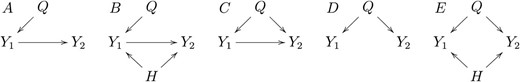
Models used in the simulation study. Y1 and Y2 represent phenotypes that co-map to the same QTL, Q. Model A represents a causal effect of Y1 on Y2. Model B represents the same, with the additional complication that part of the correlation between Y1 and Y2 is due to a hidden-variable H. Model C represents a causal-pleiotropic model, where Q affects both Y1 and Y2 but Y1 also has a causal effect on Y2. Model D shows a purely pleiotropic model, where both Y1 and Y2 are under the control of the same QTL, but one does not causally affect the other. Model E represents the pleiotropic model, where the correlation between Y1 and Y2 is partially explained by a hidden-variable H.
True and false positives
| CMST | Model A | Model B | Model C | Model D | Model E |
|---|---|---|---|---|---|
| M1 | TP | TP | FP | FP | FP |
| M2 | FP | FP | FP | FP | FP |
| M3 | FP | FP | FP | TP | FP |
| M4 | FP | FP | TP | FP | TP |
| CIT | Model A | Model B | Model C | Model D | Model E |
| M1 | TP | TP | FP | FP | FP |
| M2 | FP | FP | FP | FP | FP |
| Mi | FP | FP | TP | TP | TP |
Each entry i, j represents whether the call on row i is a true positive (TP) or as false positive (FP), when the data are generated from the model on column j. For instance, when data are generated from models A or B, a M1 call represents a true positive, whereas a M2, M3, or M4 call represents a false positive for the AIC, BIC, and CMSTs approaches (for the CIT a M2 or Mi call represents false positive). Note that a M4 call is considered a true positive for model C (in addition to model E) because it corresponds to model on Figure 1 and, hence, is distribution equivalent to model M4. Please note too that because the CIT provides P-values for only the M1 and M2 calls, but not for the M3 and M4 calls, and its output is M1, M2, or Mi, we classify a Mi call as a true positive for models C, D, and E. Observe that by doing so we are actually giving an unfair advantage for the CIT approach, since when the data are generated from, say, model E, the CIT needs only to discard models M1 and M2 as nonsignificant to detect a “true positive.” The AIC, BIC, and CMST approaches, on the other hand, need to discard models M1, M2, and M3 as nonsignificant and accept model M4 as significant.
| CMST | Model A | Model B | Model C | Model D | Model E |
|---|---|---|---|---|---|
| M1 | TP | TP | FP | FP | FP |
| M2 | FP | FP | FP | FP | FP |
| M3 | FP | FP | FP | TP | FP |
| M4 | FP | FP | TP | FP | TP |
| CIT | Model A | Model B | Model C | Model D | Model E |
| M1 | TP | TP | FP | FP | FP |
| M2 | FP | FP | FP | FP | FP |
| Mi | FP | FP | TP | TP | TP |
Each entry i, j represents whether the call on row i is a true positive (TP) or as false positive (FP), when the data are generated from the model on column j. For instance, when data are generated from models A or B, a M1 call represents a true positive, whereas a M2, M3, or M4 call represents a false positive for the AIC, BIC, and CMSTs approaches (for the CIT a M2 or Mi call represents false positive). Note that a M4 call is considered a true positive for model C (in addition to model E) because it corresponds to model on Figure 1 and, hence, is distribution equivalent to model M4. Please note too that because the CIT provides P-values for only the M1 and M2 calls, but not for the M3 and M4 calls, and its output is M1, M2, or Mi, we classify a Mi call as a true positive for models C, D, and E. Observe that by doing so we are actually giving an unfair advantage for the CIT approach, since when the data are generated from, say, model E, the CIT needs only to discard models M1 and M2 as nonsignificant to detect a “true positive.” The AIC, BIC, and CMST approaches, on the other hand, need to discard models M1, M2, and M3 as nonsignificant and accept model M4 as significant.
In the large-scale simulation study we investigate the empirical FDR (1 minus the precision) and power levels achieved by the CMST tests using the Benjamini and Hochberg (1995) and the Benjamini and Yekutieli (2001) FDR control procedures (denoted, respectively, by BH and BY), as well as no multiple testing correction. We simulate data from the models in Figure 3, which emulate eQTL hotspot patterns, i.e., genomic regions to which hundreds or thousands of traits co-map (West et al. 2007). In each simulation we generated 1000 distinct backcrosses with phenotypic data on 5001 traits on 112 individuals. We simulated unequally spaced markers for model F, but equally spaced markers for G, with Q1 and Q set 1 cM apart. Because we fit almost three million hypothesis tests in this simulation study, we did not include the CIT tests in this investigation, restricting our attention to the computationally more efficient CMST tests. The details for our choice of simulation parameters and QTL mapping are presented in File S2, File S3, and File S4. A frequent goal in eQTL hotspots studies is to determine a master regulator, i.e., a transcript that regulates the transcription of the other traits mapping to the hotspot. A promising strategy toward this end is to test the cis traits (i.e., transcripts physically located close to the QTL hotspot) against all other co-mapping traits. Our simulations evaluate the performance of the CMST tests in this setting.
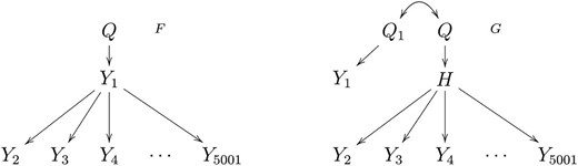
Models generating hotspot patterns. Y1 represents a cis-expression trait. Yk, k = 2, …, 5001 represent expression traits mapping in trans to the hotspot QTL Q. H represents an unobserved expression trait. Model F generates a hotspot pattern derived from the causal effect of the master regulator, Y1, on the transcription of the other traits. Model G gives rise to a hotspot pattern, due to the causal effect of H on Yk, but where the cis-trait Y1 maps to Q1, a QTL closely linked to the true QTL hotspot Q, and is actually causally independent of the traits mapping in trans to the Q.
Results
Pilot simulation study results
Figure 4 depicts the power, miss-calling error rate, and precision of each of the methods based on the simulation results of all five models in Figure 2. The results of the AIC and BIC approaches are constant across all significance levels since these approaches do not provide a measure of statistical significance. For those methods, we simply fit the models to the data and select the model with the best (smallest) score.
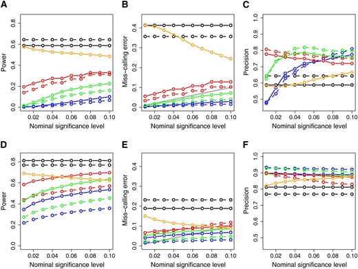
Power (A and D), miss-calling error rate (B and E), and precision (C and F) across the simulated models depicted in Figure 2. The x-axis represents the significance levels used for computing the results. (A—C) The simulations based on sample size 112; (D—F) the results for sample size 1000. Dashed and solid curves represent, respectively, AIC- and BIC-based methods. Green: parametric CMST. Red: nonparametric CMST. Blue: joint-parametric CMST. Black: AIC and BIC. Orange: CIT. The shaded line on B and E corresponds to the α levels.
Overall, the AIC, BIC, and CIT showed high power, high miss-calling error rates, and low precision. The CMST methods, on the other hand, showed lower power, lower miss-calling error rates, and higher precision. The nonparametric CMST tended to be more powerful but less precise than the other CMST approaches. As expected, for sample size 1000, all methods showed an increase in power and precision and decrease in miss-calling error rate.
Figure S3, Figure S4, Figure S5, Figure S6, and Figure S7 show the simulation results data for each one of models A to E, when sample size is 112. Figure S8, Figure S9, Figure S10, Figure S11, and Figure S12 show the same results for sample size 1000. Some of the simulated models were intrinsically more challenging than others. For instance, in the absence of latent variables the causal and independence relations can often be correctly inferred by all methods (see the results for models A and D in Figure S3, Figure S6, Figure S8, and Figure S11). However, the presence of hidden variables in models B and E tend to complicate matters. Nonetheless, although the AIC, BIC, and CIT methods tend to detect false positives at high rates in these complicated situations, the CMST tests tend to forfeit making calls and tend to detect fewer false positives (see Figure S4, Figure S7, Figure S9, and Figure S12). Model C is particularly challenging (Figure S5 and Figure S10), showing the highest false-positive detection rates among all models.
In genetical genomics experiments we often restrict our attention to the analysis of cis-genes against trans-genes. In this special case it is reasonable to expect the pleiotropic causal relationship depicted in model C to be much less frequent than the relationships shown in models A, B, D, and E, so that the performance statistics shown in Figure 4 might be negatively affected to an unnecessary degree by the simulation results from model C.
To investigate the performance of methods in the cis- against trans-case, we present in Figure 5 the simulation results based on models A, B, D, and E only. Comparison of Figures 4 and 5 show an overall improvement in power, decrease in miss-calling rates and increase in precision.
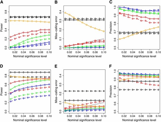
Power (A and D), miss-calling error rate (B and E), and precision (C and F) restricted to the cis- vs. trans-cases. The x-axis represents the significance levels used for computing the results. The results were computed using only the simulated models A, B, D, and E in Figure 2, since the pleiotropic causal relationship depicted in model C is expected to be much less frequent than the others when testing cis- vs. trans-case. (A–C) The simulations based on sample size 112; (D–F) the results for sample size 1000. Dashed and solid curves represent, respectively, AIC- and BIC-based methods. Green: parametric CMST. Red: nonparametric CMST. Blue: joint-parametric CMST. Black: AIC and BIC. Orange: CIT. The shaded line on B and E corresponds to the α levels.
In the analysis of trans- against trans-genes there is no a priori reason to discard the relationship depicted in model C, and more false positives should be expected. The CMST approaches, specially the joint parametric and parametric CMST methods, tend to detect a much smaller number of false positives than the AIC, BIC, and CIT approaches, as shown in Figure S5 and Figure S10.
Large-scale simulation study results
With the possible exception of the nonparametric version, the previous simulation study suggests that the CMST tests can be quite conservative. Therefore, it is reasonable to ask whether multiple testing correction is really necessary to achieve reasonable false discovery rates (FDR).
Figure 6 presents the observed FDR and power using uncorrected, BH corrected, and BY corrected P-values for the simulations based on model G. Figure 6, top, shows that, except for the AIC-based nonparametric CMST, the observed FDRs were considerably lower than the P-value cutoff, suggesting that multiple testing adjustment is not necessary for the CMST tests. Furthermore, comparison of the bottom panels shows that the BH and BY adjustments leads to a reduction in power (specially for the BY adjustment) for the joint and parametric tests at the expense of small drop in FDR levels (that were already low without any correction). For the nonparametric tests, on the other hand, BH corrections leads to bigger drops in FDR (specially for the AIC based test) and smaller drops in power. The BY correction appears too conservative even for the nonparametric tests. The results for model F are similar (Figure S13).
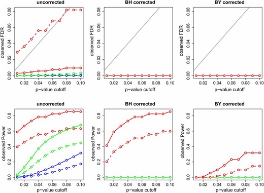
Observed FDR and power for the simulations based on model G. The x-axis represents the P-value cutoffs used for computing the results. Dashed and solid curves represent, respectively, AIC- and BIC-based methods. Green: parametric CMST. Red: nonparametric CMST. Blue: joint-parametric CMST. Black: AIC and BIC. The shaded line in the top corresponds to the α levels.
Yeast data analysis and biologically validated predictions
We analyzed a budding yeast genetic genomics data set derived from a cross of a standard laboratory strain and a wild isolate from a California vineyard (Brem and Kruglyak 2005). The data consist of expression measurements on 5740 transcripts measured on 112 segregant strains with dense genotype data on 2956 markers. Processing of the expression measurements raw data was performed as described in Brem and Kruglyak (2005), with an additional step of converting the processed measurements to normal scores. We performed QTL analysis using Haley–Knott regression (Haley and Knott 1992) with the R/qtl software (Broman et al. 2003). We used Haldane’s map function, genotype error rate of 0.0001, and set the maximum distance between positions at which genotype probabilities were calculated to 2 cM. We adopted a permutation LOD threshold (Churchill and Doerge 1994) of 3.48, controlling the genome-wide error rate of falsely detecting a QTL at a significance level of 5%.
To evaluate the precision of the causal predictions made by the methods we used validated causal relationships extracted from a database of 247 knock-out experiments in yeast (Hughes et al. 2000; Zhu et al. 2008). In each of these experiments, one gene was knocked out, and the expression levels of the remainder genes in control and knocked-out strains were interrogated for differential expression. The set of differentially expressed genes form the knock-out signature (ko-signature) of the knocked-out gene (ko-gene) and show direct evidence of a causal effect of the ko-gene on the ko-signature genes. The yeast data cross and knocked-out data analyzed in this section are available in the R/qtlyeast package at GITHUB (https://github.com/byandell/qtlyeast).
To use this information, we: (i) determined which of the 247 ko-genes also showed a significant eQTL in our data set; (ii) for each one of the ko-genes showing significant linkages, we determined which other genes in our data set also co-mapped to the same QTL of the ko-gene, generating, in this way, a list of putative targets of the ko-gene; (iii) for each of the ko-gene/putative targets list, we applied all methods using the ko-gene as the Y1 phenotype, the putative target genes as the Y2 phenotypes, and the ko-gene QTL as the causal anchor; (iv) for the AIC- and BIC-based nonparametric CMST tests we adjusted the P-values according to the Benjamini and Hochberg FDR control procedure; and (v) for each method we determined the “validated precision,” computed as the ratio of true positives by the sum of true and false positives, where a true positive is defined as an inferred causal relationship where the target gene belongs to the ko-signature of the ko-gene, and a false positive is given by an inferred causal relation where the target gene does not belong to the ko-signature.
In total 135 of the ko-genes showed a significant QTL, generating 135 putative target lists. A gene belonged to the putative target list of a ko-gene when its 1.5 LOD support interval (Lander and Botstein 1989; Dupuis and Siegmund 1999; Manichaikul et al. 2006) contained the location of the ko-gene QTL. The number of genes in each of the putative target lists varied from list to list, but in total we tested 31,975 “ko-gene/putative target gene” relationships.
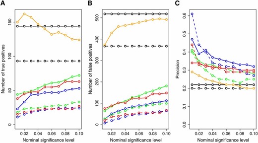
Figure 7 presents the number of inferred true positives, number of inferred false positives, and the prediction precision across varying target significance levels for each one of the methods. The CIT, BIC, and AIC had a higher number of true positives than the CMST approaches, with the AIC-based CMST methods having less power than the BIC-based CMST methods. However, the CIT, BIC, and AIC also inferred the highest numbers of false positives (Figure 7B) and showed low prediction precisions (Figure 7C). From Figure 7C we see that the CMST tests show substantially higher precision rates across all target significance levels compared to the AIC, BIC, and CIT methods. Among the CMST approaches, the joint-parametric CMST tended to show the highest precision, followed by the nonparametric and parametric CMST tests.
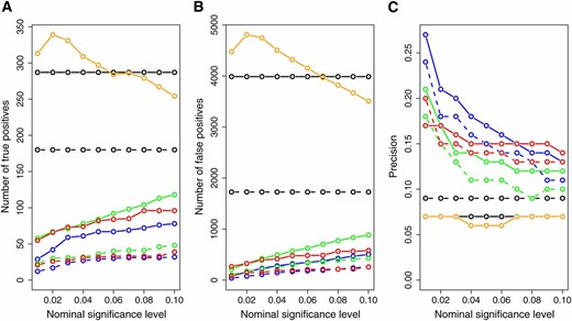
Overall number of true positives (A), number of false positives (B), and precision (C) across all 135 ko-gene/putative target lists. The x-axis represents the significance levels used for computing the results. Dashed and solid curves represent, respectively, AIC- and BIC-based methods. Green: parametric CMST. Red: nonparametric CMST. Blue: joint-parametric CMST. Black: AIC and BIC. Orange: CIT.
The results presented in Figure 7 were computed using all 135 ko-genes. However, in light of our simulation results, which suggest that the analysis of cis- against trans-genes is usually easier than the analysis of trans- against trans-genes, we investigated the results restricting ourselves to ko-genes with significant cis-QTL. Only 28 of the 135 ko-genes were cis-traits, but, nonetheless, were responsible for 2947 of the total 31,975 “ko-gene/putative target gene” relationships. Figure 8 presents the results restricted to the cis-ko-genes. All methods show improvement in precision, corroborating our simulation results. Once again, the CMST tests showed higher precision than the CIT, AIC, and BIC.
Overall number of true positives (A), number of false positives (B), and precision (C) restricted to 28 cis ko-gene/putative target lists. The x-axis represents the significance levels used for computing the results. Dashed and solid curves represent, respectively, AIC- and BIC-based methods. Green: parametric CMST. Red: nonparametric CMST. Blue: joint-parametric CMST. Black: AIC and BIC. Orange: CIT.
Discussion
In this article, we proposed three novel hypothesis tests that adapt and extend Vuong’s and Clarke’s model selection tests to the comparison of four models, spanning the full range of possible causal relationships among a pair of phenotypes. Our CMST tests scale well to large genome wide analyses because they are fully analytical and avoid computationally expensive permutation or resampling strategies.
Another useful property of the CMST tests, inherited from Vuong’s test, is their ability to perform model selection among misspecified models. That is, the correct model need not be one of the models under consideration. Accounting for the misspecification of the models is key. In general, any two phenotypes of interest are embedded in a complex network and are affected by many other phenotypes not considered in the grossly simplified (and thus misspecified) pairwise models.
Overall, our simulations and real data analysis show that the CMST tests are better at controlling miss-calling error rates and tend to outperform the AIC, BIC, and CIT methods in terms of statistical precision. However, they do so at the expense of a decrease in statistical power. While an ideal method would have high precision and power, in practice there is always a trade-off between these quantities. Whether a more powerful and less precise, or a less powerful and more precise, method is more adequate depends on the biologist’s research goals and resources. For instance, if the goal is to generate a rank-ordered list of promising candidates genes that might causally affect a phenotype of interest and the biologist can easily validate several genes, a larger list generated by more powered and less precise methods might be more appealing. However, in general, follow-up studies tend to be time consuming and expensive, and only a few candidates can be studied in detail. A long list of putative causal traits is not useful if most are false positives. High power to detect causal relations alone is not enough. A more precise method that conservatively identifies candidates with high confidence can be more appealing (see also Chen et al. 2007).
Further, the exploratory goal is often to identify causal agents without attempting to reconstruct entire pathways. Therefore, much information about the larger networks in which the tested pairs of traits reside is unknown and generally unknowable and contributes to the large unexplained variation that in turn results in low power. Our method accurately reflects this difficulty to detect causal relationships in the presence of noisy high-throughput data and poorly understood networks.
Interestingly, our data analysis and simulations also suggest that the analysis of cis-against trans-gene pairs is less prone to detect false positives than the analysis of trans- against trans-gene pairs. Our simulations suggest that model selection approaches have difficulty ordering the phenotypes when the QTL effect reaches the truly reactive gene by two or more distinct paths, only one of which is mediated by the truly causal gene (see Figure S1C, for an example).
When we test causal relationships among gene expression phenotypes, the true relationships might not be a direct result of transcriptional regulation. For instance, the true causal regulation might be due to methylation, phosphorylation, direct protein–protein interaction, transcription factor binding, etc. Margolin and Califano (2007) have pointed out the limitations of causal inference at the transcriptional level, where molecular phenotypes at other layers of regulation might represent latent variables. Model M4 (see Figure 1) can account for these latent variables and can test this scenario explicitly.
Furthermore, as pointed out by Li et al. (2010), causal inference depends on the detection of subtle patterns in the correlation between traits. Hence, it can be challenging even when the true causal relations take place at the transcriptional level. The authors point out that reliable causal inference in genome-wide linkage and association studies require large sample sizes and would benefit from: (i) incorporating prior information via Bayesian reasoning; (ii) adjusting for experimental factors, such as sex and age, that might induce correlations not explained the the causal relations; and (iii) considering a richer set of models than the four models accounted in this article.
The CMST tests represent a step in the direction of reliable causal inference in three accounts. First, they tend to be precise, declining to make calls in situations where alternative approaches usually deliver a flood of false-positive calls. Second, the CMST tests can adjust for experimental factors by modeling them as additive and interactive covariates. Third, the CMST tests can be applied to nonnested models of different dimensions and can be readily extended to incorporate a larger number of models by implementing intersection-union tests on a larger number of Vuong’s tests. For the joint-parametric test a higher-dimensional null distribution is required.
FDR control for the CMST approaches is a challenging problem as our tests violate the key assumption, made by FDR control procedures, that the distribution of the P-values under the null hypothesis are uniformly distributed (Benjamini and Hochberg 1995; Storey and Tibshirani 2003). Recall that the CMST P-values are computed as the maximum across other P-values, and the maximum of multiple uniform random variables no longer follows a uniform distribution. Additionally, the CMST tests are usually not independent since we often test the same cis-trait against several trans-traits, so that the additional assumption of independent test statistics made by the original Benjamini–Hochberg procedure does not hold. The Benjamini–Yekutieli (BY) procedure relaxes the independent test statistics assumption, and we explore both these corrections in our simulations. Our results suggest that BH and BY multiple testing correction should not be performed for the joint and the parametric CMST tests, as the FDR levels are lower than the nominal level without any correction and are too conservative with severe reduction in statistical power with the application of BH and BY control. The nonparametric CMST tests, on the other hand, seemed to benefit from BH correction, showing slight decrease in power with concomitant decrease in FDR, in spite of the nonparametric CMST tests being based on discrete test statistics and the BH procedure being developed to handle P-values from continuous statistics. Inspection of the P-value distributions (see Figure S14, Figure S15, Figure S16, and Figure S17) suggests that the smaller P-values of the nonparametric tests, relative to the other approaches, are the reason for the higher power achieved by the BH corrected nonparametric tests. The BY procedure, on the other hand, tended to be too conservative even for the nonparametric CMST tests.
The CMST approach is currently implemented for inbred line crosses. Extension to outbred populations involving mixed effects models is yet to be done. Although in this article we focused on mRNA expression traits, the CMST tests can be applied to any sort of heritable phenotype, including clinical phenotypes and other “omic” molecular phenotypes.
The higher statistical precision and computational efficiency achieved by our fully analytical hypothesis tests will help biologists to perform large-scale screening of causal relations, providing a conservative rank-ordered list of promising candidate genes for further investigations.
Acknowledgments
We thank Adam Margolin for helpful discussions and comments and the editor and referees for comments and suggestions that considerably improved this work.This work was supported by CNPq Brazil (E.C.N.); National Cancer Institute (NCI) Integrative Cancer Biology Program grant U54-CA149237 and National Institutes of Health (NIH) grant R01MH090948 (E.C.N.); National Institute of Diabetes and Digestive and Kidney Diseases (NIDDK) grants DK66369, DK58037, and DK06639 (A.D.A., M.P.K., A.T.B., B.S.Y., E.C.N.); National Institute of General Medical Sciences (NIGMS) grants PA02110 and GM069430-01A2 (B.S.Y.).
Literature Cited
Footnotes
Communicating editor: L. M. McIntyre
Author notes
Supporting information is available online at http://www.genetics.org/lookup/suppl/doi:10.1534/genetics.112.147124/-/DC1.
