


Abstract
Adaptive dynamics formalism demonstrates that, in a constant environment, a continuous trait may first converge to a singular point followed by spontaneous transition from a unimodal trait distribution into a bimodal one, which is called “evolutionary branching.” Most previous analyses of evolutionary branching have been conducted in an infinitely large population. Here, we study the effect of stochasticity caused by the finiteness of the population size on evolutionary branching. By analyzing the dynamics of trait variance, we obtain the condition for evolutionary branching as the one under which trait variance explodes. Genetic drift reduces the trait variance and causes stochastic fluctuation. In a very small population, evolutionary branching does not occur. In larger populations, evolutionary branching may occur, but it occurs in two different manners: in deterministic branching, branching occurs quickly when the population reaches the singular point, while in stochastic branching, the population stays at singularity for a period before branching out. The conditions for these cases and the mean branching-out times are calculated in terms of population size, mutational effects, and selection intensity and are confirmed by direct computer simulations of the individual-based model.
IN addition to models using quantitative genetics (Lande 1981; Barton and Turelli 1991; Iwasa et al. 1991; Pomiankowski et al. 1991), adaptive dynamics formalism has revealed diverse behaviors of evolutionary dynamics associated with continuous traits in various organisms (Metz et al. 1992; Dieckmann and Law 1996; Geritz et al. 1997, 1998). This approach allows us to analyze the evolution of many ecological traits for which frequency-dependent selection is prevalent without specifying the derlying genetic systems controlling the trait. Even in a perfectly constant environment, a population may show intriguing temporal behavior. For example, if the trait evolves by accumulation of mutations of small magnitude and if the fitness is frequency dependent, a continuous trait may show convergence to a singular point followed by spontaneous splitting of a unimodal trait distribution into a bimodal (or multimodal) one, referred to as “evolutionary branching” (Metz et al. 1992, 1996; Geritz et al. 1997). Evolutionary branching is predicted to occur at an evolutionarily singular point that is approaching stable (or convergence stable, CS) but not evolutionarily stable (ES), and it is actually observed in individual-based simulations in many models for the evolution of ecological traits.
In evolutionary branching, an evolving population spontaneously changes its trait distribution from unimodal to bimodal (or multimodal). Although evolutionary branching has been regarded as a model of sympatric speciation by some authors (Dieckmann and Doebeli 1999; Doebeli and Dieckmann 2000), the relationship between evolutionary branching in adaptive dynamics formalism and speciation events has been the focus of much debate (for review, see Waxman and Gavrilets 2005).
Most previous analyses of adaptive dynamics have assumed an infinite population size and that the fitness landscape acts as the deterministic driving force of evolution. However, in a finite population, stochastic fluctuations are unavoidable. For example, an individual with a lower fitness may be able to produce more offspring just by chance. Thus, a finite population can evolve against the selection gradient. As a result, stochasticity allows a population to jump from a low local peak to a higher peak. Hence, stochastic fluctuation can be an important factor in the outcome of evolution. The importance of stochasticity, or genetic drift, has been studied in detail in the context of quantitative population genetics (e.g., Lande 1976; Tazzyman and Iwasa 2000). On the other hand, in population genetics, random drift is known to decrease the genetic diversity of a population (e.g., Ewens 2004), which tends to slow down the action of natural selection. Hence, the effect of genetic drift is important to understand evolutionary dynamics, including evolutionary branching, in finite populations. In fact, Claessen et al. (2007) analyzed evolutionary branching in a model including three species and reported that genetic drift tends to cause a delay in evolutionary branching. However, a more detailed study of the relationship between evolutionary branching and genetic drift is needed.
In this article, we study the effect of stochastic fluctuation caused by the finiteness of population size (random genetic drift) on evolutionary branching. As an illustrative example, we adopt a model of a public goods game studied by Doebeli et al. (2004), who investigated evolutionary branching by using a corresponding individual-based simulation. The game model deals with a situation that is both biologically and socially interesting: a self-organized differentiation of players into a highly cooperative group and a noncooperative group. Concerning the genetics, we in effect assume that the population is haploid and that the focal trait is controlled by a locus with many alleles. By focusing on this simplest case, we can analyze the effect of random genetic drift on the evolutionary outcome most clearly. We first show the results of individual-based simulations, using different population sizes. We show that genetic drift is especially important when the population size is small and that evolutionary branching does not necessarily occur even when the standard theory of adaptive dynamics predicts that it should. We also derive deterministic and stochastic versions of the dynamics of the trait variance. We reveal that there are two different manners in which evolutionary branching occurs: in deterministic branching, branching may occur quickly after the population reaches the singular point, while in stochastic branching, the population stays at a singularity for a period before branching out suddenly. We derive the conditions and mean branching-out times for these cases and confirm our predictions by direct computer simulations of the individual-based model.
Evolutionary Branching in a Game in a Finite Population
Individual-based model
When the population size is infinitely large, Doebeli et al. (2004) have shown that the singular strategy is convergence stable when and evolutionarily stable when . The singular strategy is referred to as an evolutionary branching point when and . They have observed evolutionary branching in an individual-based simulation of a large population (N = 10,000).
In a finite population, the model includes random genetic drift, and the details of the updating rule and the order of different stages in population dynamics become important. Here, we assume a Wright–Fisher process. At each time step, fecundity is calculated for all N individuals. Then all individuals die and are replaced by their offspring, which are sampled multinomially, with the probability of an individual being the parent of each offspring individual proportional to the fecundity of the focal individual.
After reproduction, there is a small chance of mutation μ, and the mutant has a trait value slightly different from that of the parent. To be specific, it follows a normal distribution with a mean equal to the parent’s and a variance . Mutants are constrained to be between 0 and 1, which confines trait z within an interval [0, 1].
Evolutionary branching depends on the population size
All simulations were run with parameter values for which a unique singular point exists that is convergence stable and evolutionarily nonstable (i.e., the evolutionary branching point). Thus, evolutionary branching is expected when the population size is infinitely large.
When the population size is large (N = 8000), evolutionary branching occurs as soon as the trait evolves to reach the CS value z* (Figure 1A). For an intermediate population size (N = 1000), the population lingers around the CS value, z*, before it finally shows evolutionary branching. The waiting time until the evolutionary branching varies considerably among different simulation runs with the same parameter values (Figure 1, B and C). For a small population size (N = 200), we do not observe evolutionary branching and the population seems to stay around z*, even though z* is not evolutionarily stable (Figure 1D) (see also Wakano and Lehmann 2012).
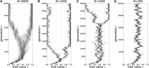
Evolutionary dynamics. (A) A simulation run with N = 8000. (B and C) Two different simulation runs with N = 1000. (D) A simulation run with N = 200. Parameters: .
The evolutionary branching dynamics are characterized by an abrupt increase or explosion of the variance of the focal phenotype (the trait variance). If all the parameters for the interactions are the same, a small population does not branch, an intermediately large population shows delayed branching, and a large population branches immediately. The intuitive reason for the smallness of the population size to suppress evolutionary branching is that genetic diversity is reduced by genetic drift every generation. In the following sections, we provide approximate dynamics for the trait variance to understand these simulation results.
Dynamics of Trait Variance
The full (individual-based) model is analytically intractable. Therefore, we derive a reduced simplified dynamical system here, which is tractable and gives predictions on the behavior of the full model. One generation in the reduced model consists of two substeps.
Substep 1: Natural selection and mutation
Substep 2: Random sampling (or random genetic drift)
Condition for the Explosion of Trait Variance
![A schematic illustration of phenotype distribution ϕ(z) and fitness function w(z) when the mean trait value z− has reached the singular strategy z*. The trait variance is Var[ϕ(z)]=m2 so the standard deviation is m2.](https://oup.silverchair-cdn.com/oup/backfile/Content_public/Journal/genetics/193/1/10.1534_genetics.112.144980/7/m_229fig2.jpeg?Expires=1716315361&Signature=axEXSZHdcsOct6gGa~iGN8GrYntmqfNVZccZnaCd9heYaixE~LJ8AjCLx2~AxuexbvhXcgy2rIte1gsxq09FrCEytNJmiFqT1CLo4HXUL962MuYFiltmCJX1FMghlVbtCXNhbSul1VAiNm2rW2AMustteZisn3VedastlIsj2Q~KWuMPlBqJM~Si74UpBiJXFFj7Jgvn0yjGoaECP17mL605V5SmXax6mMHB6rSfrDmbdr-nX-rnzjA3qf5bt8g3qwowze3Ieg6W~Nv8KT5Fhy0Guph9mw6kHKKZq19PRvLvrk9aN-o9HtfMP3sx7~-crEjXj0qV~eBjM3Yna64xeA__&Key-Pair-Id=APKAIE5G5CRDK6RD3PGA)
A schematic illustration of phenotype distribution and fitness function when the mean trait value has reached the singular strategy z*. The trait variance is so the standard deviation is .
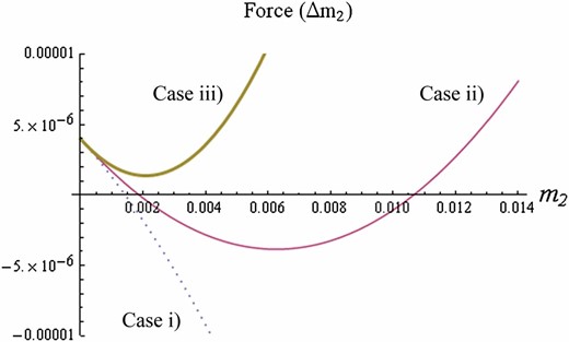
“Force” plotted against the trait variance based on Equation 10. Dotted, solid, and thick solid curves represent stabilizing selection ( = −0.2), weak disruptive selection (= 0.2), and strong disruptive selection ( = 0.6), respectively. They also correspond to cases i, ii, and iii in the main text. Parameters: N = 400, .
Combining these, we have three different cases, depending on the parameters.
- Case i: When , stabilizing selection is at work. Then the dynamics of the trait variance (Equation10) have a single positive equilibriumwhich is globally stable, and the trait variance converges to this value for any initial value. At this equilibrium, the trait variance is maintained by mutation, which increases variance, and by genetic drift and stabilizing selection, which decrease variance. Especially when the stabilizing selection is weak, trait variance converges to the level maintained by mutation–drift balance () when is small.
Case ii: When , disruptive selection is at work, but it is not very strong. Then the dynamics of the trait variance have two positive equilibria: the smaller one is stable, but the larger one is unstable. If the trait variance starts from a small value, it converges to the smaller equilibrium, where the trait variance is maintained mainly by the mutation–drift balance. If the trait variance starts from a larger value, then disruptive selection dominates, leading to the unlimited growth of the trait variance.
Case iii: When , disruptive selection is strong. The dynamics of the trait variance no longer have a stable equilibrium. Starting from any initial value, the trait variance keeps increasing without limit.
Figure 4 shows a bifurcation diagram of the variance dynamics given by Equation 10, with the stabilizing/disruptive selection coefficient () as a bifurcation parameter. Figure 5 shows a bifurcation diagram in which the population size (N) is a bifurcation parameter. We have a similar bifurcation diagram where mutational effects () serve as a bifurcation parameter (not shown). We regard the explosion of the trait variance in the dynamics of Equation 10 as evolutionary branching. Then, these bifurcation diagrams show that evolutionary branching occurs as a result of a saddle-node bifurcation. Evolutionary branching is predicted to occur at a non-ES singular point when disruptive selection intensity, population size, mutation rate, and mutation step size are sufficiently large. Specifically, the deterministic dynamics of Equation 10 predict that evolutionary branching occurs when holds.
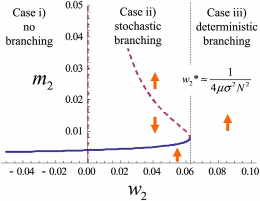
Stable (solid) and unstable (dashed) branches of the trait variance with disruptive selection intensity as a bifurcation parameter. Arrows indicate the direction of systematic change in . Parameters: N = 1000, .
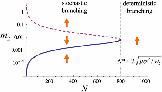
Stable (solid) and unstable (dashed) branches of the trait variance with population size N as a bifurcation parameter. A Log plot is shown. Arrows indicate the direction of systematic change in . Parameters: .
Stochastic Calculation of the Explosion of Variance
The deterministic dynamics of the trait variance represented by Equation 10 indicate only the expectation of one-generational change. There must be stochasticity caused by the genetic drift. Results of an individual-based model, such as those illustrated in Figure 1, clearly show stochasticity. To account for stochasticity, the deterministic difference of Equation 10 needs to be modified by an additional term. In this section, we derive the stochastic differential equation model considering the stochasticity of trait variance dynamics.
The second term on the right-hand side of Equation 12 represents stochasticity in trait variance caused by random genetic drift (see Appendix C for derivation). The stochastic fluctuation term depends on the trait variance itself (geometric Brownian motion), because the amplitude of fluctuation in the trait variance in each generation of offspring is large when the trait variance in each parental generation is large. The stochastic term also depends on population size, because fluctuation is averaged out in large populations. Hence, random genetic drift becomes less important in larger populations. The system is similar to but different from the motion of a particle moved by force shown in Figure 3 under heat noise.
Stationary distribution
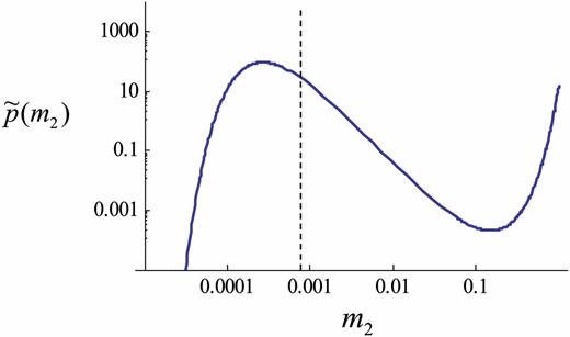
The stationary distribution of the trait variance (Equation 14). A Log-Log plot is shown, and thus the probability density is much higher at the peak than it appears. The locally stable value of the variance according to Equation 11 is 0.00081, which is close to = 0.0008 (dashed line). Note that a local peak lies at a value <0.0008 because of geometric Brownian motion. Parameters: N = 200, .
Comparison with the results of simulations:
We compared the stationary distribution of the trait variance between the theoretical prediction given by Equation 14 and the observed distribution obtained from the individual-based simulation (Evolutionary Branching in a Game in a FinitePopulation section). Figure 7 shows good agreement between the diffusion approximation (i.e., the SDE model) and the corresponding simulation result with a small population size. In particular, the approximation captures the shift of the mode—the peak of the distribution lies at the value smaller than . The average trait variance in an interval shown in Figure 7 is close to for both analytic prediction (Equation 14) and simulation results.
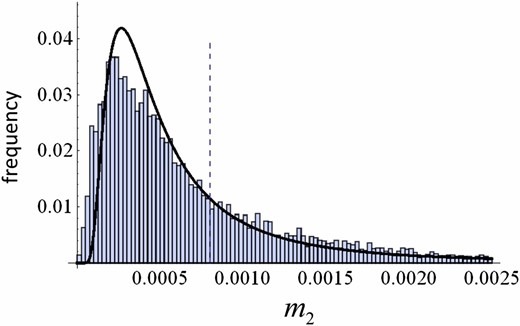
The stationary distribution of the trait variance . Curves represent an analytic result (Equation 14), while bars are a histogram of realized trait variances in a simulation run for time steps. The dashed line represents = 0.0008. In the simulation, the initial trait distribution was set as monomorphic at z = 0.2. The transition from this initial state to the stationary state was negligible as it took only ∼5000 time steps. Parameters: N = 200, .
Waiting time for evolutionary branching
In case ii, there are stable and unstable equilibria for the trait variance, the latter being larger than the former. If the initial value of trait variance is smaller than the unstable equilibrium, the deterministic model Equation 11 predicts that variance would be maintained indefinitely. In contrast, if the initial value is larger than the unstable equilibrium, it quickly increases and grows without limit. Hence, whether trait variance eventually explodes depends on the initial condition. In the presence of stochasticity, however, the trait variance would not be maintained at smaller values than the unstable equilibrium; instead, it would fluctuate around the stable equilibrium for a period, but then eventually increase beyond the unstable equilibrium and diverge to infinity. Hence, under the stochastic differential equation, the trait variance is predicted to explode eventually even if the initial value is small. The timing of this explosion is controlled by the stochasticity.
The mean waiting time prior to explosion is a typical “first passage time” problem in diffusion theory. This has also been used in calculating the mean time of fixation in population genetics (Kimura and Ohta 1968) and the mean time to extinction in conservation biology (e.g., Lande 1993; Hakoyama and Iwasa 2000) and physiology (e.g., Ricciardi and Smith 1977).
Comparison with the results of simulations:
We compared the mean waiting times observed in the computer simulations of the individual-based model and the prediction by the approximate stochastic differential equation model given by Equation 16. Once the system reaches a convergence stable point, the trait variance is expected to be close to the locally stable value (see also our results on stationary distribution). Thus, we numerically calculate and compare the corresponding result in individual-based simulation (Figure 8). We also derive the probability distribution of the first passage time by using Kolmogorov’s backward equation in Appendix E, but the fit of the shape of the probability distribution of waiting times to the distribution observed in individual-based simulations is less than perfect (Figure 9).
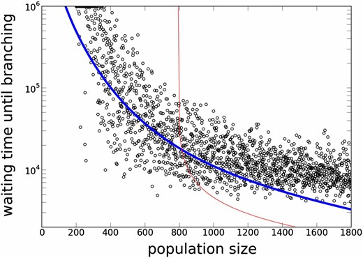
A Log plot of waiting times for evolutionary branching for different population sizes (N). The thick and thin curves represent analytic results based on a SDE model (Equation 16) and those based on an ODE model (Equation 11), respectively. Each open circle represents the result of a single run in individual-based simulation. The first time the trait variance exceeded 0.1 is shown. In the simulation, the initial trait distribution was set as monomorphic at z = 0.2 and each run consisted of time steps. Simulation runs in which the variance did not explode are plotted at . Time required to reach a singular point in the simulation was ∼5000 when N = 200 and ∼2000 when N = 1800, which is included to show open circles. Thus, open circles are expected to lie slightly above the curve. Parameters: .
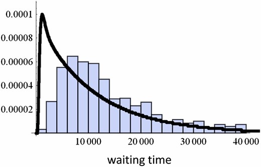
The distribution of waiting times. Curves represent an analytic result (see Appendix E), while bars represent a histogram of the waiting time obtained in 1000 different runs of individual-based simulation. Parameters: N = 1000, .
As we decrease N, the waiting time increases exponentially, and it eventually becomes impossible to escape from the locally stable unimodal state in a reasonable time (Figure 8). This implies that evolutionary branching is unlikely to occur in a small population.
When N is very large, genetic drift can be neglected and the system is approximated by the ODE: . Thus, the waiting time can be approximated by the time required to move from to the right boundary . This time is ∼1500 for N = 1000 and ∼960 for N = 2000. This calculation, in conjunction with Figure 8, shows that the stochastic fluctuation plays a dominant role even in a population of 1000 individuals.
Our reduced model measures genetic diversity in trait distribution. An alternative measure of genetic diversity is the number of segregating alleles, which depends only on μ and is predicted by Ewens’ sampling formula when selection is absent (Ewens 2004). Figure 10 shows the effect of mutation rate μ and mutation step size . Simulations confirmed our prediction that only the value of matters, even though the numbers of segregating alleles in the simulation with N = 1800 were ∼50 and ∼150 for and 0.01, respectively. It is also confirmed that smaller mutational effects require a longer waiting time until evolutionary branching.
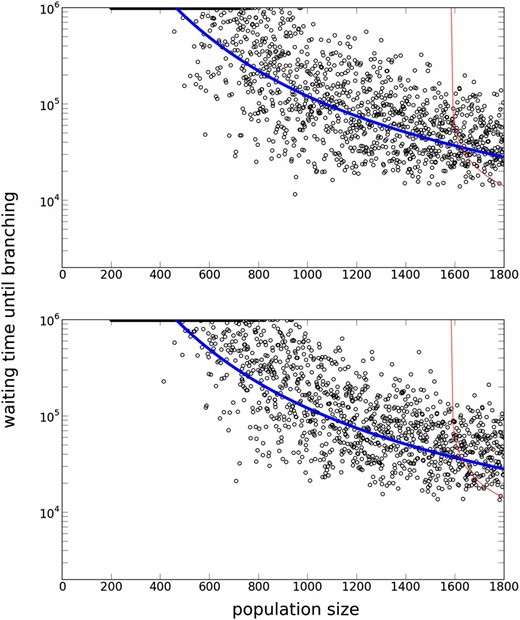
A Log plot of waiting times for evolutionary branching for different population sizes and mutation parameters. The top panel () depicts a result for a smaller mutation rate than in Figure 8, while the bottom panel () depicts a result for a smaller mutation step size. As is the same, the analytic prediction curves are the same. The two simulation results are also undistinguishable. Parameters: .
Discussion
In this article, we have studied the effect of stochastic fluctuation due to finite population size on evolutionary branching. We have derived an ordinary differential equation and then a stochastic differential equation for the dynamics of trait variance. The analysis has revealed that there are two different manners in which evolutionary branching occurs: deterministic branching and stochastic branching. In the case of deterministic branching, evolutionary branching occurs relatively soon after the mean trait reaches the branching point. This occurs when disruptive selection intensity exceeds a threshold value, , which can be approximated by . This condition for deterministic branching implies that the intensity of random genetic drift is smaller than disruptive selection intensity and the mutational effects (see later in article). If the opposite inequality holds, i.e., when disruptive selection is weaker than the threshold, then a unimodal distribution is locally stable in the deterministic model and stochastic fluctuation is necessary for the population to undergo evolutionary branching. We call this latter type of evolutionary branching “stochastic branching.” We observed a relatively long waiting time until evolutionary branching occurs in simulations. The distribution and expectation of the waiting time were mathematically calculated and these predictions were consistent with computer simulations of the individual-based model. Considering the several assumptions we have adopted, the consistency is better than expected, although not perfect. As population size or mutational effect decreases, the waiting time exponentially increases. Mathematically, this is because these factors appear in the exponent in the expression of the expected waiting time (Equation 16). Although the increase of the waiting time is a continuous phenomenon resulting from the underlying stochasticity in individual-based simulations, we can understand evolutionary branching by classifying it as either deterministic branching in which stochastic fluctuation is unnecessary or stochastic branching in which stochastic fluctuation is necessary.
Our analysis has revealed that evolutionary branching is almost impossible in some biological situations in which the effective population size or mutational effect is sufficiently small. As a population size increases, our condition for deterministic evolutionary branching approaches and converges to the standard branching-point condition. The condition can be written as , which can be used as an approximate indicator; for example, a population with size N = with mutational effects is predicted to show deterministic branching when disruptive selection intensity is , although such individual-based simulation is almost impossible.
To mimic the full individual-based model by using the deterministic and stochastic equations of the trait variance, we have adopted several simplifying assumptions in deriving the dynamics: i.e., trait distribution is assumed to be close to normal, and the trait variance is small enough to justify series expansion. From simulation results, it is clear that the trait distribution finally becomes multimodal when evolutionary branching occurs. Thus, our analytic results are valid only for the initial growth of the trait variance where unimodal distribution (approximated by a normal distribution) becomes broader at the singular point. This initial explosion is followed by highly nonlinear and complex dynamics that realize a multimodal distribution. Nevertheless, the agreement of our analytic prediction and simulation results suggests that our reduced model captures the onset of evolutionary branching.
Based on individual-based simulations, Claessen et al. (2007) reported delayed evolutionary branching and proposed two reasons: random genetic drift and extinction of incipient branches. In contrast to Claessen et al. (2007), our model has no fluctuation in the total population size. Thus, the delayed or absent evolutionary branching is caused by demographic stochasticity—the fluctuation in the number of offspring each individual produces. Our simple model has enabled us to derive the condition for evolutionary branching mathematically, with random genetic drift taken into consideration, which has been only verbally proposed before. In addition, our mathematical analysis and simulation results have revealed that the mutation rate and step size are as important as population size.
In this article, to illustrate the effect of genetic drift on the evolutionary branching, we used as an example a pairwise interaction game that incorporated a Wright–Fisher update. We conjecture that the extension of our model to include a Moran update or to a multiplayer game is readily possible. In the case of including a Moran update, the loss of genetic diversity (Equation 7) should be appropriately modified and also the unit of time should be rescaled since N Moran steps correspond to a single Wright–Fisher step. The result of our model should be easily extended to resource-competition models, which have been intensively studied in adaptive dynamics (e.g., Dieckmann and Doebeli 1999; Sasaki and Dieckmann 2011; Mirrahimi et al. 2012).
We have focused on the dynamic processes in which the population escapes from the locally stable value of the trait variance, while keeping its trait distribution as a unimodal distribution. Conceptually, if we allow all possible trait distributions, we might have two locally stable states, one of which corresponds to a unimodal state and a second that corresponds to a fully branched state. Stochastic branching in the present model considers only the case in which a system located at the unimodal state escapes from this local optimum by stochastic fluctuation (random genetic drift). However, a branched state can also evolve back to the unimodal state by genetic drift; thus, a stochastic analysis including both escaping from and evolving back to the unimodal distribution would give us an even deeper understanding of evolutionary branching.
Acknowledgments
We thank the following people for their very helpful comments: C. Hauert, Y. Kobayashi, C. Miura, W. Nakahashi, H. Ohtsuki, and A. Sasaki. This work was supported by Japan Science and Technology Precursory Research for Embryonic Science and Technology (J.Y.W.), by a Grant-in-Aid for Scientific Research (B) from Japan Society for Promotion of Science (to Y.I.), and also by the support of the Environment Research and Technology Development Fund (S9) of the Ministry of the Environment, Japan.
Literature Cited
Footnotes
Communicating editor: W. Stephan
