


Abstract
The effective population size (Ne) is notoriously difficult to accurately estimate in wild populations as it is influenced by a number of parameters that are difficult to delineate in natural systems. The different methods that are used to estimate Ne are affected variously by different processes at the population level, such as the life-history characteristics of the organism, gene flow, and population substructure, as well as by the frequency patterns of genetic markers used and the sampling design. Here, we compare Ne estimates obtained by different genetic methods and from demographic data and elucidate how the estimates are affected by various factors in an exhaustively sampled and comprehensively described natural brown trout (Salmo trutta) system. In general, the methods yielded rather congruent estimates, and we ascribe that to the adequate genotyping and exhaustive sampling. Effects of violating the assumptions of the different methods were nevertheless apparent. In accordance with theoretical studies, skewed allele frequencies would underestimate temporal allele frequency changes and thereby upwardly bias Ne if not accounted for. Overlapping generations and iteroparity would also upwardly bias Ne when applied to temporal samples taken over short time spans. Gene flow from a genetically not very dissimilar source population decreases temporal allele frequency changes and thereby acts to increase estimates of Ne. Our study reiterates the importance of adequate sampling, quantification of life-history parameters and gene flow, and incorporating these data into the Ne estimation.
THE effective population size (Ne) is an essential concept in evolutionary and conservation biology as it determines the strength of stochastic evolutionary processes relative to deterministic forces (Crow and Kimura 1970). In the absence of gene flow, the rate of loss of genetic diversity via genetic drift is greater in populations with small Ne. The effective population size is, however, notoriously difficult to accurately estimate in wild populations as it is influenced by a number of parameters that are difficult to characterize in natural systems. A number of different methods have been developed for estimating Ne, and these are affected variously by different processes at the population level such as immigration, fluctuations in population size, population substructure, and life-history characteristics. When possible, it is therefore important to compare Ne estimates obtained using different methods and elucidate how different processes affect the various methods for Ne estimation (Fraser et al. 2007).
Two main types of approaches have been used to estimate Ne: genetic and demographic. Genetic methods attempt to infer the magnitude of the effective population size by characterizing the genetic consequences of limited population size, whereas demographic methods depend upon measurement of demographic parameters that have theoretically been shown to influence Ne. The most common genetic approach is the so-called temporal method (Waples 1989). It is based on measurements of the amount of random genetic drift between generations that is inversely proportional to the effective population size (Nei and Tajima 1981). Although this method typically makes the simplifying assumption that generations are discrete, it is routinely applied also to species with overlapping generations. Overlapping generations are expected to bias Ne estimates because temporal fluctuations in allele frequencies follow more complicated patterns when generations overlap (Jorde and Ryman 1995). Especially relevant is to explore short-term genetic fluctuations, as researchers are often interested in obtaining an estimate of Ne without having to sample a population interval several generations apart, which would be impractical, especially in long-lived organisms. With overlapping generations the amount of allele frequency change depends not only on the true effective size and the time between samples, but also on what population units are being sampled (e.g., single cohorts or aggregates of multiple cohorts) and the life-history parameters (age-specific birth and survival rates) linking these units to the effective size of the population under consideration (Jorde and Ryman 1995). Such complications underscore the need for empirical Ne studies founded on detailed knowledge of the organism’s life history and age structure, to validate the various genetic estimation methods.
When generations overlap, an alternative to estimate the usual, per generation, effective size (Ne) is to focus on a single breeding season and estimate the per-season effective number of breeders (Nb) (sensuWaples 1990). In most real populations Nb will be less than the number of sexually mature individuals because of larger than binomial variance in family sizes. In semelparous organisms (i.e., species that breed only once and die immediately after), Ne is simply the sum of Nb over a generation. It is, however, unclear how these two effective numbers relate in the more common iteroparous (repeat breeders) situation and it is thus useful to estimate both numbers for such species.
Most wild populations will be at least partially connected to other conspecific populations by migration. The resulting gene flow will contribute to the genetic constitution of the recipient population and affect the estimated Ne. Difficulties in measuring Ne also arise from the lack of adequately accounting for the spatial and metapopulation structure and clarity on how these affect Ne. Depending on the variation in size and productivity of subpopulations and the patterns of migration and extinction/recolonization rates, the sum of Ne’s of the subpopulations can either be greater or smaller than the effective size of the total (meta)population (NeT) (Nunney 1999; Palstra and Ruzzante 2011). With high levels of dispersal, the concept of a (sub)population Ne becomes increasingly meaningless since it is not acting as an independent unit (Nunney 2000). Fragmented populations may instead form dynamic nonequilibrium metapopulation systems with reduced total effective size (NeT) (Hedrick and Gilpin 1997). Quantifying all these effects is often difficult and our knowledge of the effective size in natural populations is consequently limited.
The sampling scheme itself can have pronounced effects on estimates of Ne. Sampling issues need to be considered carefully when applying a particular estimator for Ne, as different estimators make different assumptions on the structure of data and the conditions under which individuals are collected. For genetic methods, precision is restricted by sampling limited numbers of individuals and genes. Bias may result from improper sampling of the population and unbiased estimates of allele frequencies require representative samples of individuals from each age class, which is rarely obtained from natural populations. In systems where migration occurs, it is also important that samples are drawn from the entire population and not only from subunits of the population (Nei and Tajima 1981; Waples 1989). Also, for the demographic methods representative offspring sampling is crucial for obtaining accurate estimates of family size variation. Accurate estimation of Ne thus requires careful consideration of a number of sources for potential errors.
In this study, we compare different Ne estimates in a semiisolated resident brown trout population for which age-specific fertility and survival, as well as gene flow, have been estimated. The system has been thoroughly sampled from 2002 to 2006 and all sampled fish have been aged and genotyped. We could thus obtain allele frequency estimates for five annual (multicohort) samples and for eight consecutive single cohorts (1998–2006), and we used these to estimate genetic drift and effective size. In addition, we have a demographic Ne estimate (Serbezov et al. 2011) calculated from a parentage analysis study (Serbezov et al. 2010) for this population. Thus, we can compare the demographic Ne estimate with various genetic estimates presented herein. Specifically, we compare the demographic Ne estimate with genetic estimates obtained by using a method specifically developed for organisms with overlapping generations (Jorde and Ryman 1995), a method based on short-term genetic changes but also allowing for gene flow (Wang and Whitlock 2003), a method based on the relationship between randomly generated linkage disequilibrium and the effective population size (Hill 1981; Waples and Do 2008), and a maximum-likelihood coalescent-based method (Beaumont 2003). The comparison of several methods applied to data from this comprehensively described system allows us to assess how various population processes affect Ne estimates in natural populations.
Materials and Methods
Brown trout
Brown trout (Salmo trutta) mate in fresh water and the eggs are commonly deposited in clean gravel (redds) in running water by the female. After hatching and depletion of yolk-sac reserves, the alevins emerge from the gravel and establish feeding territories, facing a period of high mortality risk (Elliott 1994). During later life stages, some trout remain in their natal stream whereas others migrate to larger systems—rivers, lakes, or the ocean to feed—and then home to their natal habitat to breed.
Study site and data collection
Brown trout were sampled from a small forest stream, Bellbekken (Figure 1), in southeast Norway (N 61.15°, E 11.51°) during the period 2002–2006 (see Carlson et al. 2008 and Serbezov et al. 2010 for detailed information on the stream and the sampling procedure). Briefly, a 1.5-km stretch of the stream was divided into 25 contiguous sections that were electrofished systematically and thoroughly during early summer (June) and autumn (late September to early October), starting in autumn 2002 and ending in autumn 2006. The downstream section starts at a small waterfall (section 1 below the waterfall, sections 2–25 above the waterfall), which should prevent upstream migration under most conditions, leading to weak but significant genetic differentiation between trout upstream and downstream the waterfall (Taugbøl 2008). Below the waterfall the stream enters the larger river Julussa. To map all potential sources of migration to Bellbekken we also sampled trout outside the focal 1.5-km study area (Figure 1). Specifically, during 2005 and 2006 brown trout were sampled from four additional sites: (1) at the confluence between Julussa and Bellbekken (n = 77 trout), (2) 2.6 km upstream in Julussa (n = 51), (3) 4.5 km downstream in Julussa (n = 61), and (4) 1.5 km upstream in Bellbekken (n = 48). Tissue samples were taken noninvasively from all fish, and individuals in Bellbekken were aged, sexed if mature, and marked as described previously (for details, see Serbezov et al. 2010).
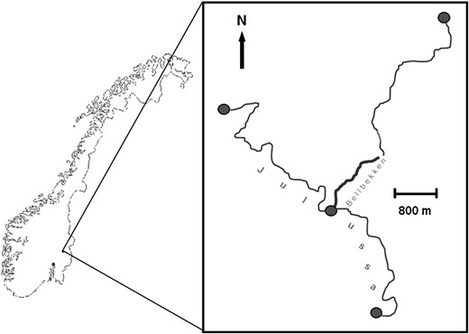
Overview of the sampled locations. Bellbekken (1504 m) was exhaustively sampled in the period 2002–2007. Samples from a location 1450 m upstream of the focal area were collected in 2006 and from three locations in the larger river Julussa in 2005 and 2006 (shaded circles).
Genetic analysis
All sampled fish (in total 4441 individuals) were analyzed with 15 microsatellite loci (details of DNA extraction and the PCR amplification can be found in Serbezov et al. 2010). The 15 loci were tested for null alleles with the Microchecker (Van Oosterhout et al. 2004) and CERVUS (Marshall et al. 1998) software packages, and no null alleles were found. The year–site–loci samples did not show any systematic deviations from Hardy–Weinberg expectations and <10% of the samples were significant at the 5% level of confidence without allowance for multiple tests. Many of these were due to heterozygosity excesses, indicating that they are not caused by null alleles. Twelve percent of all individuals were genotyped more than once, allowing us to estimate the genotyping and scoring error rates (see Serbezov et al. 2010). We used Arlequin v3.1 (Excoffier et al. 2007) to quantify the spatial and temporal components of the genetic variance. This was done by regarding the consecutive (autumn) samples (from 2002 to 2006) as the temporal source of variation and the stream sections (2–25) as the spatial source of variation.
Population structure and migration
We used STRUCTURE 2.3.3 (Pritchard et al. 2000) to estimate the total number of populations in the pooled material from Julussa and Bellbekken. The Julussa sample was made up of all fish sampled there in the fall 2005 and 2006 (total of 213 individuals), and the Bellbekken sample consisted of the same number of individuals, randomly chosen from the Bellbekken fall 2005 sample. The optimal number of populations (K) was determined from ΔK likelihood evaluations (Evanno et al. 2005). As two distinct populations were inferred (see Results), we identified migrants into Bellbekken using GENECLASS2 (Piry et al. 2004). We conducted the assignment using the Bayesian probability method (Rannala and Mountain 1997) and Monte Carlo resampling for probability testing with 10,000 simulated individuals (type-I error, α = 0.01).
The genealogical history of alleles in Bellbekken and the larger Julussa was inferred considering two alternative models of population structure: a genetic drift model and a gene flow model. The drift model is that of an ancestral, panmictic population that has split into two isolated populations that diverge by random genetic drift alone. The gene flow model, on the other hand, assumes that the gene frequencies in the two populations are determined by a balance between genetic drift and gene flow (migration). Gene flow depends on the effective number of migrants, Nem (Ne being the effective population size and m is the fraction of the population exchanged per generation), whereas the amount of drift depends on t/Ne, where t is the time since separation of the two populations. The 2mod software (Ciofi et al. 1999) calculates the likelihood of each model on the basis of averaging over all possible values of Nem and t/Ne.
Ongoing gene flow and migration rates were also estimated using BAYESASS v1.3 (Wilson and Rannala 2003). This Bayesian method uses the fact that immigrants show temporal linkage disequilibrium in their genotypes relative to members of the hosting population, thus allowing their identification as recent (first or second generation) immigrants.
Demographic estimates of Ne
Demographic estimates of Ne were obtained using expressions derived by Hill (1972, 1979) and described in Serbezov et al. (2011). Briefly, we obtained estimates of variance in life-time reproductive success in Bellbekken by using an individual-based model using empirical estimates of sex- and age-specific reproductive success (Serbezov et al. 2010) and age-specific survival rates (Carlson et al. 2008). Age-specific maturation probabilities were also modeled on empirical data (Serbezov et al. 2011). By tracking each member of the cohort throughout its life, the model directly incorporates age structure in the mean and variance of life-time reproductive success and does so without assuming stable age distribution. This model was also run on a subset of the data after removing all individuals that were assigned as potential immigrants from Julussa.
Temporal methods for estimating Ne
The effective population size (Ne) of the brown trout population in the Bellbekken stream was also estimated from temporal variance in microsatellite allele frequencies. Four different data sets were used, i.e., annual samples of all individuals caught in Bellbekken, with and without individuals assigned as putative migrants, and all individuals belonging to the same cohort, again with and without potential immigrants (Table 1). Because sampling was noninvasive and fish were marked and returned after sampling, a large number of individuals appear in more than one of the annual samples, whereas individuals were counted only once when constructing the cohort data sets (cf. the larger sums of annual samples than cohort samples in Table 1). Separate analyses of samples with and without potential immigrants should counteract the consequences of the assumption of most methods of a single, isolated, population receiving no immigrants over the study interval. Most of the methods described below also assume, in addition to the population being closed to immigration, that generations are discrete and do not overlap. It is problematic to apply these methods to age-structured populations, such as the brown trout considered here, and for some methods it is not clear exactly what is being estimated from different groupings of the data (annual samples or cohorts). As annual samples are easier to obtain, most applications of these methods in the literature seem to be based on such “annual” samples and count the number of generations between samples (fractions of a generation in our case).
The number of sampled brown trout from Bellbekken at each fishing episode and the number of fish belonging to one of eight consecutive cohorts
| Sample size | Assigned as immigrants from Julussa | Sample size (excluding immigrants) | |
|---|---|---|---|
| Fishing episode | |||
| Fall 2002 | 741 | 105 | 636 |
| Spring 2003 | 499 | 62 | 437 |
| Fall 2003 | 591 | 56 | 535 |
| Spring 2004 | 1051 | 79 | 972 |
| Fall 2004 | 1018 | 97 | 921 |
| Spring 2005 | 1017 | 75 | 942 |
| Fall 2005 | 1103 | 98 | 1005 |
| Spring 2006 | 631 | 41 | 590 |
| Fall 2006 | 512 | 49 | 463 |
| Cohort | |||
| 1998 | 166 | 16 | 150 |
| 1999 | 333 | 31 | 302 |
| 2000 | 340 | 66 | 274 |
| 2001 | 267 | 40 | 227 |
| 2002 | 740 | 49 | 691 |
| 2003 | 823 | 53 | 770 |
| 2004 | 703 | 49 | 654 |
| 2005 | 288 | 23 | 265 |
Exhaustive sampling was carried out twice each year (fall and spring) from 2002 to 2006, and scale readings or body length was used to classify fish to year of birth (i.e., cohort). Potential immigrants from Julussa (Figure 1) were identified using GENECLASS v2 on the basis of statistical assignment to reference sample (n = 325) from the Julussa river.
| Sample size | Assigned as immigrants from Julussa | Sample size (excluding immigrants) | |
|---|---|---|---|
| Fishing episode | |||
| Fall 2002 | 741 | 105 | 636 |
| Spring 2003 | 499 | 62 | 437 |
| Fall 2003 | 591 | 56 | 535 |
| Spring 2004 | 1051 | 79 | 972 |
| Fall 2004 | 1018 | 97 | 921 |
| Spring 2005 | 1017 | 75 | 942 |
| Fall 2005 | 1103 | 98 | 1005 |
| Spring 2006 | 631 | 41 | 590 |
| Fall 2006 | 512 | 49 | 463 |
| Cohort | |||
| 1998 | 166 | 16 | 150 |
| 1999 | 333 | 31 | 302 |
| 2000 | 340 | 66 | 274 |
| 2001 | 267 | 40 | 227 |
| 2002 | 740 | 49 | 691 |
| 2003 | 823 | 53 | 770 |
| 2004 | 703 | 49 | 654 |
| 2005 | 288 | 23 | 265 |
Exhaustive sampling was carried out twice each year (fall and spring) from 2002 to 2006, and scale readings or body length was used to classify fish to year of birth (i.e., cohort). Potential immigrants from Julussa (Figure 1) were identified using GENECLASS v2 on the basis of statistical assignment to reference sample (n = 325) from the Julussa river.
The “standard” temporal method:
Maximum-likelihood coalescent-based method:
This method makes the same assumption of no mutations, no selection, no migration, and discrete generations, as the standard temporal method. Likelihood-based estimators are generally considered superior to the method-of-moments estimators (i.e., those relying on estimated amount of genetic drift, F) in that they are apparently less sensitive to recent departures from migration–drift equilibrium (Tallmon et al. 2004). In addition, in populations with low Ne that do not follow the Wright–Fisher model (finite N, random mating and nonoverlapping generations), the gene genealogy might be better approximated by the coalescent (Berthier et al. 2002). We implemented this method with the TMVP software package developed by Beaumont (2003) for annual and cohort samples. It incorporates Bayesian prior information by making the user specify a maximum Ne (we used Ne max = 1000), resulting in a uniform prior distribution of Ne from 0 to Ne max.
Maximum-likelihood method [MLNE (Wang and Whitlock 2003)]:
Methods used to estimate Ne will be biased if the effects of immigration on allele frequencies are large relative to the effect of genetic drift. In addition to running all models with and without putative immigrants, we evaluated the impact of gene flow on Ne by applying Wang and Whitlock’s (2003) model incorporated in the MLNE software package, which jointly estimates Ne and the rate of gene flow (m). This method is based on a pseudo-maximum–likelihood approach and uses temporal gene frequency changes in the focal population and the allele frequency of the potential source population to estimate effective size and migration rate separately. The method assumes that there is no selection and negligible mutation, that the source population is sampled, that allele frequencies in the source population and in the immigrants are stable, and that sampling does not affect the availability of reproductive individuals (Wang and Whitlock 2003).
Accounting for age structure:
To estimate the correction factors C and G we first used the field data to estimate annual survival (li) and birth (bi) rates for each age class (i). Age-specific survival rates were estimated from capture–mark–recapture data on brown trout in Bellbekken (Carlson et al. 2008). On the basis of estimated “winter” and “summer” season survival, age-specific monthly survival probabilities were estimated, and we used these estimates to calculate an average survival rate per year, S = 0.41. This estimate was subsequently used to calculate li = Si−1, where i is the age class, counted from 1 (l1 = 1 per definition).
There was, however, some uncertainty in the age determination based on scales. In Bellbekken fish growth is slow and adjacent scale rings are often difficult to distinguish. A number of individuals that were not marked at first capture, or had lost their tags, were genotyped more than once and, as they had identical genotypes and compatible body length measurements, provided an estimate of the age-determination error rate. It was found that 36.5% of the fish that were aged ≥3 years were underestimated by 1 year and 19.0% were underestimated by 2 years. A corrected age distribution was obtained by iterating a computer simulation procedure in which 1 or 2 years are randomly added to the age of individual fish, in concurrence with the estimated proportions. Accordingly, age-specific birth rates (bi) were estimated in two steps. First, the probability of being mature at age i, prob(mature(i)), was estimated by fitting a logistic regression of the individual’s age on its maturity index (a binomial response variable). Second, the average number of offspring produced by parents of age i (age counted when their offspring were born, the following spring) was estimated on the basis of parentage assignment analysis from genetic data (Serbezov et al. 2010). We used a log-linear model to relate the age of the spawners to the number of assigned offspring. Because the slope (b) of this regression was estimated for log-transformed data, the untransformed estimate is noffspring(i) = ib, where b is the (unweighted) mean of the estimated slopes for each sex. Finally, we estimated age-specific birth rates, bi = prob(maturei) × offspringi, which were normalized to yield a constant population size, by dividing by ∑li × bi. In both models, the logistic and log-linear, the uncertainty in the aging of the fish was accounted for by iterating the procedure described above 1000 times, and we used the median values (slope) from the simulated iterations.
The resulting li and bi values (Table 2) were used to estimate average generation length, G = ∑li × bi × i, and correction factor C by iterating Equations 10–13 in Jorde and Ryman (1995) and substituting into their Equation 23 (using software “factorc”, available from http://folk.uio.no/ejorde). We arrived at estimates of C = 10.70 and G = 5.73 years. Finally, the effective size per generation, Ne, was estimated from allele frequency data from consecutive cohorts according to Equation 2, using data with and without putative immigrants.
Estimated survival (li) and fecundity (bi) rates for each age class used to calculate the correction factor (C) and generation interval (G) for brown trout in Bellbekken
| Age class | li | bi |
|---|---|---|
| 1 | 1 | 0 |
| 2 | 0.4100 | 0 |
| 3 | 0.1681 | 0.46 |
| 4 | 0.0689 | 2.12 |
| 5 | 0.0283 | 8.02 |
| 6 | 0.0116 | 21.15 |
| 7 | 0.0048 | 36.03 |
| 8 | 0.0019 | 46.50 |
| 9 | 0.0008 | 53.64 |
| Age class | li | bi |
|---|---|---|
| 1 | 1 | 0 |
| 2 | 0.4100 | 0 |
| 3 | 0.1681 | 0.46 |
| 4 | 0.0689 | 2.12 |
| 5 | 0.0283 | 8.02 |
| 6 | 0.0116 | 21.15 |
| 7 | 0.0048 | 36.03 |
| 8 | 0.0019 | 46.50 |
| 9 | 0.0008 | 53.64 |
| Age class | li | bi |
|---|---|---|
| 1 | 1 | 0 |
| 2 | 0.4100 | 0 |
| 3 | 0.1681 | 0.46 |
| 4 | 0.0689 | 2.12 |
| 5 | 0.0283 | 8.02 |
| 6 | 0.0116 | 21.15 |
| 7 | 0.0048 | 36.03 |
| 8 | 0.0019 | 46.50 |
| 9 | 0.0008 | 53.64 |
| Age class | li | bi |
|---|---|---|
| 1 | 1 | 0 |
| 2 | 0.4100 | 0 |
| 3 | 0.1681 | 0.46 |
| 4 | 0.0689 | 2.12 |
| 5 | 0.0283 | 8.02 |
| 6 | 0.0116 | 21.15 |
| 7 | 0.0048 | 36.03 |
| 8 | 0.0019 | 46.50 |
| 9 | 0.0008 | 53.64 |
Linkage disequilibrium method for estimating Ne [LDNE (Waples and Do 2008)]
In addition to generating temporal change in allele frequencies (i.e., random genetic drift), a limited effective size has other genetic consequences, including fluctuating associations of alleles at different loci (gametic phase or “linkage” disequilibrium). In an isolated population of constant size and stable structure, the amount of linkage disequilibrium (LD) can thus be used to measure Ne (Hill 1981). This method has advantages, such as requiring only a single sample of individuals. Like other methods it depends on a number of assumptions, in addition to those in common with the temporal methods above, also that loci are physically unlinked and independently segregating. Estimates of effective population size were obtained from annual samples and from single cohorts. Although to our knowledge this method has not been evaluated for age-structured species with overlapping generations, it is assumed that annual samples from the entire population should yield an estimate of per-generation Ne, whereas single-cohort data should characterize the effective number of breeders (Nb) per spawning season (cf. Fraser et al. 2007). We therefore did not apply any corrections for overlapping generations to this method. The method was also applied to data excluding putative immigrants.
The sibship assignment method for estimating Nb [COLONY v2.0 (Wang 2009)]
This is a hybrid approach with features of both the demographic and the genetic approaches. First, on the basis of a sample of individuals from a single cohort in the population, sibship assignments among cohort members are obtained from multilocus genotype data. These assignments are then used to calculate half-sib and full-sib probabilities and then estimate Ne. This method assumes a population with discrete, nonoverlapping generations and, when it is applied to a sample of individuals taken at random from a single cohort in a population with overlapping generations, is supposed to give an estimate of the Nb that have produced this cohort. Wang (2009) suggested that this method for Nb estimation should be applicable to populations with either discrete or overlapping generations, random or nonrandom mating, and that it can be applied to estimate Nb in subpopulations with immigration (Wang 2009). The method is, however, fairly new and has to our knowledge not been extensively evaluated either in practical application or with computer simulations.
Results
We successfully genotyped 3805 individual brown trout from Bellbekken belonging to eight consecutive cohorts (1998–2005), with at least 166 individuals from each (Table 1, Figure 2A). In addition, we genotyped 325 fish coming from different locations in the Julussa river (including station 1 from Bellbekken, which is below the waterfall and hence part of Julussa).
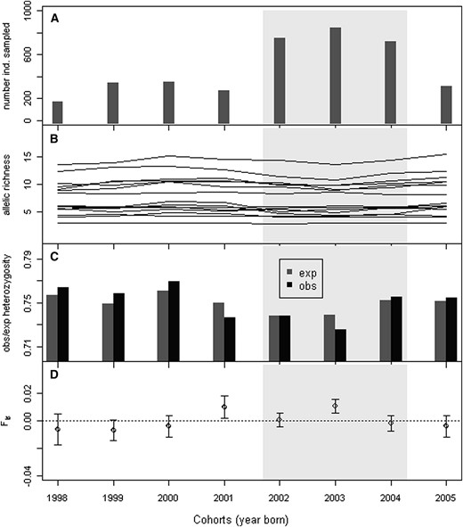
Characteristics for the eight consecutive cohorts of brown trout (Salmo trutta) sampled from Bellbekken. (A) The number of individuals sampled from each cohort. (B) Allelic richness of all 15 loci used in the analyses. (C) Expected and observed heterozygosity. (D) Inbreeding coefficient (Fis). The zone with light shading marks the three cohorts for which we have estimated variance of individual reproductive success on the basis of parentage assignment analysis and used it for calculating a “demographic” estimate of Ne.
The number of alleles per locus over all samples ranged from 3 to 22 (mean = 11.9). The frequency of the most common allele ranged from 0.20 to 0.61 (mean = 0.35). Although the most common allele within a locus did change and there was some allele turnover, the allele frequency distribution was relatively stable across cohorts and there seemed to be no loss of rare alleles, leading to relatively stable temporal allelic richness values (El Mousadik and Petit 1996) (Figure 2C). The average observed heterozygosity in the eight consecutive cohorts was also very stable (0.73–0.76), but two of the eight cohorts had significantly positive Fis values (Figure 2D).
Population structure and gene flow
The temporal genetic variation among annual samples of brown trout in Bellbekken accounted for 0.02% and spatial differentiation accounted for 0.04% of the total genetic variation. An analysis of all pooled samples within Bellbekken showed a pattern of isolation by distance (β = 0.5, r2 = 0.25, P < 0.05) (L. A. Vøllestad, D. Serbezov, A. Bass, L. Bernatchez, E. M. Olsen, and A. Taugbøl, unpublished results).
Using STRUCTURE, the pooled material from Bellbekken and Julussa was best grouped into two populations (K = 2). Bellbekken was moderately, but significantly, genetically differentiated from the larger Julussa (Fst = 0.018, P < 0.05). The population structure analysis overwhelmingly supported the gene flow model [p(gene flow model) = 1].
Gene flow estimates between Bellbekken and Julussa are summarized in Table 3. The short-term gene flow estimates between Bellbekken and the “upstream” location obtained with BAYESASS were highly asymmetrical, with higher values in the Bellbekken upstream direction, compared to the other way around. Thus we chose, also considering the small sample size in the upstream location and the results from STRUCTURE, to treat Bellbekken and Julussa as a system of two populations that exchange genes, ignoring the sample from the upstream location. There was a high degree of congruence between short-term migration rate estimates between Bellbekken and Julussa obtained with BAYESASS and the MLNE estimate based on annual data.
Estimated ongoing migration rates (m) of brown trout in and out of Bellbekken, based on Wang and Whitlock (2003) MLNE and Wilson and Rannala (2003) BAYESASS methods
| Method | Parameter estimated | Estimate (95% C.I.) |
|---|---|---|
| MLNE: annual samples | m in Bellbekken | 0.0083 (0.0082–0.0115) |
| MLNE: cohort samples | m in Bellbekken | 0.0746 (0.0614–0.0904) |
| BAYESASS | m in Bellbekken from Julussa | 0.012 (0.006–0.020) |
| BAYESASS | m in Julussa from Bellbekken | 0.019 (0.003–0.046) |
Demographic method
The effective population size estimate (NeV) based on the variance in lifetime reproductive success was 104 [with a 95% confidence interval (C.I.) from 44 to 215]. The effective number of breeders per season obtained from empirical estimates of yearly reproductive success (Serbezov et al. 2012) ranged between 43 and 53 for the 3 consecutive years studied.
Temporal methods for Ne estimation
Estimates based on consecutive cohorts:
There was a consistent pattern of allele frequency change between cohorts (Figure 3), with highest Fs values observed at 3 years difference. For consecutive cohorts that were used to estimate effective size, the average Fs over loci was 0.01151, with a standard error (SE) of 0.00112. Using an average estimate of C/G = 1.87 (C = 10.70, G = 5.73) in Equation 2, this corresponds to an estimated effective size per generation of Ne = 81 (Table 4) for the Bellbekken brown trout population. There are two important sources of uncertainty in this point estimate. The first is the stochastic variation due to the limited sample sizes and number of screened loci. This uncertainty is quantified by the SE of Fs and a 95% C.I. for Ne from this effect is ∼C/(G × 2 × (Fs ± 1.96 × SE)) or 68–101 (Table 4). Second, there is an uncertainty, and undoubtedly also natural variation, in the demographic parameters, leading to uncertainty in the calculated factor C/G. A sensitivity analysis, varying demographic parameters (the annual survival rate and the slope of the logistic regression of number of offspring on parent age) around their point estimates, indicated that this ratio could vary between 1.52 and 2.00 over the likely parameter space (Figure 4). Taking this range as an indication of uncertainty in the estimated C/G ratio, the “confidence interval” for Ne would widen to ∼55–107. This is a moderate adjustment to the original confidence interval and we have not included it in the results tabulated in Table 4.
![Allele frequency differences [Fs, adjusted for sampling (Jorde and Ryman 2007, Equation 13)] between pairs of cohorts (born 1998–2002) of brown trout in Bellbekken. The year in each plot refers to birth (hatching) year of the cohort that is being compared to subsequent cohorts (e.g., the 1998 cohort is compared to cohorts born in 1999, 2000, and up to 2005, seven comparisons altogether). Vertical bars refer to 95% confidence intervals for the point estimated, calculated by jackknifing over loci.](https://oup.silverchair-cdn.com/oup/backfile/Content_public/Journal/genetics/191/2/10.1534_genetics.111.136580/10/m_579fig3.jpeg?Expires=1716351929&Signature=zaBSs4u7OARYHQ1Fwpz4GXcPgFtnDV-M0tlSL2u3ll2V8bgwvLcRyNh1zR2Lt7f2gVn11p4wsCEj085p3UZGLfp7fD8oKr~424eIfyRVxuEEONKKF8jfXFSe3i6uWUz4G3GpyvdWNQh13RkATVqORRZxY3F4L4Abqp5jPpQmNPLgUcz2bVsRJiTcJXJ3A~3P~Pqgxj5X1NMS5CGbfhXdxkFFY9iTnnmDyxU42aCapJq1Nscx~IFcV6G6TsNcOe~HIRFcPY1zgMjdJGIq6-QpiSfId1yVjS7Fafyw1KRnTqIX3KHYsSU1FHTccFXEWJzYdi-SbpZGaFGWRvI9mlC2XA__&Key-Pair-Id=APKAIE5G5CRDK6RD3PGA)
Allele frequency differences [Fs, adjusted for sampling (Jorde and Ryman 2007, Equation 13)] between pairs of cohorts (born 1998–2002) of brown trout in Bellbekken. The year in each plot refers to birth (hatching) year of the cohort that is being compared to subsequent cohorts (e.g., the 1998 cohort is compared to cohorts born in 1999, 2000, and up to 2005, seven comparisons altogether). Vertical bars refer to 95% confidence intervals for the point estimated, calculated by jackknifing over loci.
Estimated per-generation and seasonal effective sizes of brown trout in Bellbekken by different methods and data
| All individuals | Excluding immigrants | ||||
|---|---|---|---|---|---|
| Method | Correctiona | Nx | 95% C.I. | Nx | 95% C.I. |
| Estimates of per-generation Ne | |||||
| Data: consecutive annual (autumn) samples | |||||
| Moments, Fk (Pollak 1983) | 1/G | 121 | 89–176 | 106 | 77–153 |
| Moments, Fs (Jorde and Ryman 2007) | 1/G | 81 | 58–143 | 69 | 47–128 |
| ML, closed (Wang and Whitlock 2003) | 1/G | 127 | 106–154 | NA | |
| ML, open (Wang and Whitlock 2003) | 1/G | 106 | 89–130 | NA | |
| Coalescent (Beaumont 2003) | 1/G | 87 | 66–111 | 91 | 69–117 |
| Data: single annual (autumn) samples | |||||
| LD (Waples and Do 2008) | None | 100 | 58–142 | 93 | 53–132 |
| Data: consecutive cohort samples | |||||
| Moments, Fk (Pollak 1983) | C/G | 105 | 93–117 | 103 | 90–115 |
| Moments, Fs (Jorde and Ryman 2007) | C/G | 81 | 68–101 | 78 | 65–98 |
| ML, closed (Wang and Whitlock 2003) | C/G | 326 | 305–351 | NA | |
| ML, open (Wang and Whitlock 2003) | C/G | 221 | 206–237 | NA | |
| Coalescent (Beaumont 2003) | C/G | 141 | 128–144 | 143 | 135–144 |
| Data: demographic (Serbezov et al. 2010) | |||||
| Lifetime Vk (Hill 1979) | None | 104 | 44–215 | 96 | 45–205 |
| Estimates of effective number of breeders Nb | |||||
| Data: single cohort samples | |||||
| LD (Waples and Do 2008) | None | 53 | 22–84 | 52 | 17–87 |
| Sibship (Wang and Whitlock 2003) | None | 56 | 15–97 | NA | |
| Data: demographic (Serbezov et al. 2010) | |||||
| Seasonal Vk | None | 40 | 32–49 | 31 | 27–35 |
Consecutive annual samples yield an estimate of drift per year. The tabulated estimates of per-generation effective size (Ne) were calculated by multiplying the annual estimate by 1/G (Hill 1979, Equation 4), where G = 5.73 is the average generation length. For consecutive cohorts the estimate refers to temporal allele frequency shifts among cohorts, and Ne estimates have been corrected by multiplying by the factor C/G or 1.87 (Equation 2). Estimates of per-season effective number of breeders (Nb: LD, sibship, and demographic methods only) were not adjusted. C.I. is the 95% confidence interval for the point estimates, either as given directly by the respective software or as calculated from standard errors for the relevant statistic (F or 1/2Ne), assuming normal distributed statistics, and was corrected with 1/G or C/G as for the corresponding point estimate.
| All individuals | Excluding immigrants | ||||
|---|---|---|---|---|---|
| Method | Correctiona | Nx | 95% C.I. | Nx | 95% C.I. |
| Estimates of per-generation Ne | |||||
| Data: consecutive annual (autumn) samples | |||||
| Moments, Fk (Pollak 1983) | 1/G | 121 | 89–176 | 106 | 77–153 |
| Moments, Fs (Jorde and Ryman 2007) | 1/G | 81 | 58–143 | 69 | 47–128 |
| ML, closed (Wang and Whitlock 2003) | 1/G | 127 | 106–154 | NA | |
| ML, open (Wang and Whitlock 2003) | 1/G | 106 | 89–130 | NA | |
| Coalescent (Beaumont 2003) | 1/G | 87 | 66–111 | 91 | 69–117 |
| Data: single annual (autumn) samples | |||||
| LD (Waples and Do 2008) | None | 100 | 58–142 | 93 | 53–132 |
| Data: consecutive cohort samples | |||||
| Moments, Fk (Pollak 1983) | C/G | 105 | 93–117 | 103 | 90–115 |
| Moments, Fs (Jorde and Ryman 2007) | C/G | 81 | 68–101 | 78 | 65–98 |
| ML, closed (Wang and Whitlock 2003) | C/G | 326 | 305–351 | NA | |
| ML, open (Wang and Whitlock 2003) | C/G | 221 | 206–237 | NA | |
| Coalescent (Beaumont 2003) | C/G | 141 | 128–144 | 143 | 135–144 |
| Data: demographic (Serbezov et al. 2010) | |||||
| Lifetime Vk (Hill 1979) | None | 104 | 44–215 | 96 | 45–205 |
| Estimates of effective number of breeders Nb | |||||
| Data: single cohort samples | |||||
| LD (Waples and Do 2008) | None | 53 | 22–84 | 52 | 17–87 |
| Sibship (Wang and Whitlock 2003) | None | 56 | 15–97 | NA | |
| Data: demographic (Serbezov et al. 2010) | |||||
| Seasonal Vk | None | 40 | 32–49 | 31 | 27–35 |
Consecutive annual samples yield an estimate of drift per year. The tabulated estimates of per-generation effective size (Ne) were calculated by multiplying the annual estimate by 1/G (Hill 1979, Equation 4), where G = 5.73 is the average generation length. For consecutive cohorts the estimate refers to temporal allele frequency shifts among cohorts, and Ne estimates have been corrected by multiplying by the factor C/G or 1.87 (Equation 2). Estimates of per-season effective number of breeders (Nb: LD, sibship, and demographic methods only) were not adjusted. C.I. is the 95% confidence interval for the point estimates, either as given directly by the respective software or as calculated from standard errors for the relevant statistic (F or 1/2Ne), assuming normal distributed statistics, and was corrected with 1/G or C/G as for the corresponding point estimate.
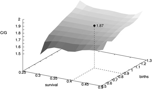
Sensitivity analysis of the correction factor C/G over a range of demographic parameter values, for brown trout in Bellbekken. “Survival” is the annual survival rate (assumed to be constant for each age) and “births” refers to the slope of the logistic regression of number of offspring on parent age. The range of demographic values used in the analysis is a generous interpretation of the uncertainties of the estimated values given in Table 2. The solid circle at C/G = 1.87 is the value that was used when estimating Ne from temporal allele frequency shifts among consecutive cohorts.
Compared to the Fs-based method, the Fk- and the ML-based methods yielded somewhat higher estimates of Ne when based on consecutive cohort data and adjusted with the factor C/G (cf. Table 4). These ranged from the standard temporal method (Pollak 1983) estimate of 105 to 326 for the ML method of Wang and Whitlock (2003), with an intermediate estimate of 141 for the coalescent method of Beaumont (2003).
Estimates based on annual samples:
Annual (autumn) samples of mixed-age composition contain partially overlapping sets of individuals, as many individuals appear in >1 year and consequently fluctuated considerably less in allele frequencies over time than did cohort samples. The amount of allele frequency change from year to year (Fs, calculated from all consecutive pairs of years) averages 0.0011 (SE = 0.00024) or only approximately 1/10th the magnitude of cohort fluctuations (0.0115: see above). We used only the autumn samples when estimating annual drift and Ne, as also including spring samples would complicate the analyses of drift without contributing much in the way of new data as most individuals that were sampled in the spring were also found in the autumn samples. On the basis of the estimated annual drift among consecutive annual autumn samples, the two moments-based methods yielded estimates of Ne [adjusted for generation length by multiplying with 1/G (Hill 1979, Equation 4)] of 121 and 81, both very similar to the corresponding estimates based on cohort data (105 and 81, respectively; Table 4). Indeed, all methods were found to yield fairly similar results for annual data, ranging from 87 for the coalescent method to 127 for the ML method. These all compare well with the previously demographic estimate of Ne = 104 (95% C.I. = 44–215) for this brown trout population. In the case of annual samples, however, the confidence intervals for the point estimates are typically broader than those based on cohort data.
Estimates of effective number of breeders, Nb:
Estimates obtained using linkage disequilibrium data based on cohorts (i.e., single-year classes) were on average about half the magnitude of the corresponding estimate of Ne based on annual data (mean ± 95% C.I. = 56.1 ± 18.8 vs. 101.0 ± 20.4, t-test = 4.7, d.f. = 15, P = 0.0003; Table 4; Figure 5) The only other method that gave an estimate of Nb, the sibship method, gave a very similar point estimate of 53. Both genetic estimates are thus in fair agreement with, but slightly higher than, the previous demographic estimate of the effective number of breeders per season of 40 (Table 4) for this population.
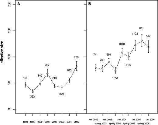
Estimates of effective population size (Ne) of brown trout in Bellbekken based on linkage disequilibrium (LD) data. Shown are (A) estimates (with 95% C.I.) based on year cohorts were born in eight successive spawning seasons (1998–2006), and (B) estimates based on all individuals caught in nine consecutive fishing episodes (fall 2002 to fall 2006). The numbers next to the plotted points are the number of individuals (n) the estimates are based on.
The effect of gene flow on estimated Ne
The procedures for estimating Ne and Nb were repeated on reduced data sets (annual samples or cohorts) with individuals identified by GENECLASS v2.0 as potential migrants removed (6.8% of all individuals were removed). There was no difference in the estimated proportion of immigrants between the sexes (test for equality of proportions: χ2 = 1.6, d.f. = 1, P = 0.2). Removing putative migrants resulted in somewhat lower effective population size estimates for all methods (2–16% for different methods), except for the coalescent method that yielded very similar estimates with and without immigrants (cf. Table 4). Randomly removing the same number of individuals as the number of putative immigrants did not change the Ne estimates obtained using these methods (data not shown), indicating that the slight reduction seen in the other methods is an effect, although modest, of immigration and not of reduced sample sizes.
Discussion
In this study we have investigated short-term genetic changes in an exhaustively sampled and demographically mapped stream-resident brown trout population. Despite relatively small population size, we documented high levels of genetic diversity and no evidence of inbreeding. We then estimated the short-term effective population size (Ne) using different genetic methods, all based on a number of assumptions, and compared the results with an estimate obtained using demographic data (Serbezov et al. 2011). There was broad congruence among estimates based on different genetic methods, as well as between genetic and demographic estimates. Some effects of violating the assumptions of the different methods were nevertheless apparent, as discussed below.
Genetic variation and genotypic frequencies
Low-frequency alleles were the most common allele frequency class, indicating that the population had not undergone any recent severe bottleneck. This was also confirmed by the fact that bottleneck tests were negative (results not shown). Also, the allele frequency distribution did not change significantly during the eight consecutive brood years studied, indicating a relatively stable number of spawners contributing each season. There did not seem to be any reduction of allele richness or level of heterozygosity, indicating that there were no inbreeding processes in our system during the period studied (8 consecutive brood years), most likely as a result of ongoing gene flow from the larger river Julussa. That gene flow is a major factor preserving genetic variability is suggested by the fact that most of the populations of brown trout that have been reported to display a low degree of genetic variation are from systems where immigration is restricted; i.e., the population is either physically isolated or located in the uppermost part of the drainage (Marshall et al. 1992; Prodohl et al. 1997; Carlsson and Nilsson 2001). In addition, the apparent demographic stability and the flexible mating system that involves both polygamy and iteroparity (Serbezov et al. 2010) would further help preserve the number of alleles and the high levels of heterozygosity.
Distribution of genetic variation in time and space
The temporal genetic variation of brown trout in Bellbekken accounted for 0.02% of the genetic variability. This result is comparable to a previous study of brown trout, also based on a short time span [0.03% (Ryman 1983)]. The degree of spatial differentiation accounted for 0.04% of the total variation. This is approximately the same value as the one estimated in another study of brown trout within pairs of interconnected lakes with apparently high levels of gene flow (Ryman et al. 1979). Nevertheless, there was no clear indication that our stream-resident population is divided into lasting subpopulations. Analysis of the 2002–2004 cohorts revealed that although there can be some significant Fst values between the 24 sections of the stream, this differentiation is not consistent between years (data not shown). Also, there was no consistent significant heterozygote deficiency relative to the Hardy–Weinberg genotypic proportions at any locus, and indeed there were a number of cases of heterozygote excess, the opposite of what is expected from population subdivision. The occasional significant Fst values are apparently a result of a large proportion of the sample being from a stream section that consists of offspring belonging to the same family before they have dispersed. Brown trout offspring from a family do tend to cluster together in Bellbekken until their second summer (L. A. Vøllestad, D. Serbezov, A. Bass, L. Bernatchez, E. M. Olsen, and A. Taugbøl, unpublished results), although offspring belonging to the same families could be found all over the stream (Serbezov et al. 2010). Because of the lack of a permanent substructure, we treat our target as a single population. However, as discussed by Nei and Tajima (1981), the effect on the Ne estimates of sampling more than one genetically distinct population depends on the sampling strategy: if all populations are proportionately represented, the estimated effective size will be that of the total (combined) population. Our intensive and spatially uniformly distributed sampling should make sure that this is achieved to a satisfactory degree.
The magnitude of the Fs values, the amounts of allele frequency change obtained from annual samples, increased rather constantly between years (data not shown). This pattern indicates that we are indeed monitoring genetic drift in this study, as potentially confounding processes such as fluctuating selection, migration, and nonrandom sampling [e.g., kin sampling (Allendorf and Phelps 1981; Hansen et al. 1997)] are not expected to result in a linear increase with time. Also, in the cohort data, even though it hardly covers one brown trout generation, a consistent pattern of low Fs values was observed at about one generation (5.73 years) and a high value at 3 years (about half a generation) (cf. Figure 3). These patterns are in agreement with the theoretical expectations for selectively neutral alleles (cf. Jorde 2012) and observations lend support to the presumption that the main cause of the observed allele frequency changes is limited effective population size, i.e., genetic drift.
Assumptions of genetic methods of estimating Ne
Genetic methods have been employed to circumvent the need to estimate Ne from demographic data. All such methods, however, make a variety of assumptions that are almost always broken to some degree. All assume no mutation or selection on the markers used in the analyses. As our study covers a very short period of time, hardly covering a single generation, we can safely ignore the effect of mutation. The markers used in this study also do not seem to be under selection. In general, however, these methods also include several of the following assumptions: (i) adequate sample sizes or number of loci utilized, (ii) knowledge of the extent of gene flow as well as knowledge of source populations contributing migrants, (iii) no population size fluctuations over the period Ne was estimated, (iv) discrete generations, and (v) sufficient number of generations separating temporal samples. Violation of these assumptions could lead to a bias in the estimates. Nevertheless, the approximate congruence between most estimates suggests that we have arrived close the “true” Ne value using these methods. Slight exceptions to the general congruence are the estimates obtained by the ML method of Wang and Whitlock (2003) and to a lesser extent the coalescent method of Beaumont (2003), when using cohort sample data. Possibly, the adjustment for overlapping generations, by multiplication with C/G, is not appropriate for these methods. This issue needs further study.
Despite the general congruence among most methods and data sets, some effects of violating underlying assumptions are apparent. For example, assuming a closed population when the focal population is not completely isolated is seen to affect systematically all methods and tends to bias estimates of Ne upward (except for the coalescent approach, Table 4). Removing putative immigrants or applying the only method specifically allowing for immigrants (the ML method) led to a reduced estimate of Ne, by a modest 2–16%. Bias introduced by uncritical adoption of the discrete generation model to age-structured species with overlapping generations could also bias estimates (Waples and Yokota 2007; Palstra and Ruzzante 2008; Waples et al. 2011). In this case bias depends on what population segments are being sampled, and we investigated two scenarios: sampling of single, consecutive cohorts and annual, multicohort samples. In either case similar, and presumed unbiased, estimates can be obtained (Table 4) if measurements are appropriately adjusted (employing correction factors C/G and 1/G, respectively). Failure to adjust estimates would lead to corresponding bias. Bias with cohort samples arises mainly because the signals of genetic drift will strongly be affected by the pattern of allele frequency covariance among cohorts generated by age structure (Jorde and Ryman 1995; Jorde 2012). This pattern depends on the population’s survival (li) and fecundity (bi) values (Table 2), but the resulting C/G surface is quite flat over a wide range of parameter values (cf. Figure 4) and the Ne estimates are consequently little affected by the exact magnitude of these life-history values. Hence, studies lacking adequate data for estimating local demographic parameters may nevertheless use this method to correct bias by adopting published values from conspecific populations (cf. Jorde and Ryman 1996; Heggenes et al. 2009).
The most commonly used measures of allele frequency change, Fc (Nei and Tajima 1981) and Fk (Pollak 1983), tend to be downward biased (thus biasing upward the Ne estimates), when allele frequencies are close to zero or unity (Waples 1989). This bias was systematically characterized by Jorde and Ryman (2007) and an alternative estimator was proposed (Fs). Although there is a trade-off between accuracy and precision when selecting estimators for genetic drift and effective size for the temporal method, computer simulations have shown that the Fs estimator yields unbiased estimates compared to those based on Fc and Fk estimators (Jorde and Ryman 2007). In our results, the Fk (and Fc; data not shown)-based estimates gave indeed higher values than those based on the unbiased Fs (Table 4). This is probably so because allele frequencies in our study are not uniformly distributed, as would usually be the case in data from natural systems. Hence, the Ne value obtained by the Fs temporal method is probably closer to the true Ne value. On the other hand, the cohort model for iteroparous species may also underestimate Ne if there is a correlation between reproduction and future survival (Jorde and Ryman 1995). This is apparently because the variance in lifetime reproductive success is reduced (and true Ne therefore increases) as fewer breeders can reproduce more than once. Simulation studies show that this is indeed the case for our system (Serbezov et al. 2011), and this might explain why the moments-based estimates from cohort data are somewhat lower than the rest. Also, genetic estimates of Ne derived from models for overlapping generations are sensitive to the confidence with which individuals have been assigned to their respective cohorts, on the basis of age determination from fish scales. Random errors in the assignment will likely introduce an upward bias into Ne, since a mixture of individuals of different ages in the presumed cohort will dilute the signals of genetic differentiation actually present among the cohorts. This might be the case in our study for older individuals (Serbezov et al. 2011).
The precision of the Ne estimates depends on the strength of the drift signal relative to sample noise. In species with overlapping generations these signals would be stronger between consecutive cohorts, compared to (mixed-age) samples between consecutive years. Consequently, the estimates obtained using cohort data typically had narrower confidence limits compared to the estimates obtained using annual samples (cf. Table 4).
We obtained Ne estimates from the LD method that were similar to those of the other methods and to the estimate based on demographic data (cf. Table 4). Recent theoretical and simulation results indicate that immigrants are expected to increase estimated Ne from this method, but only slightly so (Waples and England 2011). This prediction was confirmed in our empirical estimates that, as in most other methods, were a little lower with immigrants removed from the data (cf. Table 4). Moreover, the nine consecutive temporal samples gave rather congruent estimates: the Ne values all fell within the rather narrow range from 74 to 131. Our results thus suggest that the LD method of estimating Ne gives plausible estimates, at least when based on sufficiently large samples, and the validity of the estimates is confirmed by replicate temporal sampling. In the case of sufficient sampling, temporal replication of the LD method can be used to evaluate potential changes in Ne for genetic monitoring, and the effective size seemed to be quite stable over the study interval for the Bellbekken population (Figure 5).
Gene flow and its effect on estimated Ne
In this study, we have analyzed genetic changes in a system where all potential gene flow source populations have been mapped and sampled. There was congruence in m estimates obtained using the Wilson and Rannala (2003) estimate and the Wang and Whitlock (2003) ML estimate based on annual sample data (m ≈ 0.01, Table 3). The ML estimate based on cohort sample data was higher (m ≈ 0.07) and, as discussed in connection with the Ne estimates, there may be problems with applying the ML method to such cohort data. Computer simulations will be useful for exploring this issue in more detail.
Current analytical limitations complicate investigating the effects of gene flow on Ne over short time spans. Nevertheless, by removing potential immigrants from the Ne calculation with the temporal methods, the LD method (Waples and Do 2008), although not the coalescent method (Beaumont 2003), resulted in slightly lower Ne estimates than the ones obtained on the basis of allele frequencies from all individuals sampled in Bellbekken (cf. Table 4). Wang and Whitlock (2003) have argued that, over few generations, migration increases allele frequency changes relative to change due to drift alone but, over many generations, migration has the opposite effect of stabilizing allele frequencies. Fraser et al. (2007) argued that, even in the short term, migration from a genetically similar population would not necessarily increase allele frequency change relative to drift alone. In the present situation, we found that including immigrants in the data set led to a slight decrease in the allele frequency change and a corresponding increase in estimated Ne (cf. Table 4). Similarly, the Ne-CLOSED (no migration) estimates were correspondingly higher than the Ne-OPEN (with migration) ones from the ML method (Wang and Whitlock 2003). Although this method assumes constant migration from an infinite source of fixed allele frequency, which is hardly the case in any natural systems, including ours, this does not seem to affect much our Ne or m estimates, possibly because migration was low. Environmental instability, fluctuations in demography, and life-history variation are likely factors influencing patterns of gene flow in a system. To fully understand the impact of gene flow on evolutionary dynamics of a system it is important to consider how gene flow varies over short and longer time spans (Hare et al. 2011).
Conclusions
Many genetic methods have been proposed to estimate Ne (and Nb) in natural populations and these make somewhat different assumptions regarding population and sample characteristics. On the basis of a comprehensive sampling effort in a natural brown trout population system, our findings demonstrate general congruence among estimates obtained by the various genetic methods and from demographic data. This congruence raises confidence in the general usefulness of genetic estimates of effective population size, also when the underlying assumptions are not fully met, as is almost always the situation with natural populations. The strength of the present study is in the extensive sampling effort, yielding relatively narrow confidence intervals for point estimates and thus allowing meaningful comparison among methods. Obviously, the true Ne is not known in this or other natural populations, and computer simulations with known Ne will be useful for evaluating methods over a wider range of parameter values. The present empirical study adds realism to such evaluations and provides a useful point of departure for future computer simulations.
A data file with the microsatellite genotypes, as well as the age and the place individuals were sampled, used in the analyses in this article is freely available at http://dx.doi.org/10.5061/dryad.44pm4pq6.
Acknowledgements
We thank the large number of graduate students that have participated in fieldwork over the years. The large amount of laboratory work would have been impossible without the kind assistance of Lucie Papillon, Vicky Albert, and Annette Taugbøl. We thank an anonymous reviewer for valuable comments. We thank the Norwegian Research Council for financial support.
Literature Cited
Footnotes
Communicating editor: M. A. Beaumont
