


Abstract
Range expansions cause a series of founder events. We show that, in a one-dimensional habitat, these founder events are the spatial analog of genetic drift in a randomly mating population. The spatial series of allele frequencies created by successive founder events is equivalent to the time series of allele frequencies in a population of effective size ke, the effective number of founders. We derive an expression for ke in a discrete-population model that allows for local population growth and migration among established populations. If there is selection, the net effect is determined approximately by the product of the selection coefficients and the number of generations between successive founding events. We use the model of a single population to compute analytically several quantities for an allele present in the source population: (i) the probability that it survives the series of colonization events, (ii) the probability that it reaches a specified threshold frequency in the last population, and (iii) the mean and variance of the frequencies in each population. We show that the analytic theory provides a good approximation to simulation results. A consequence of our approximation is that the average heterozygosity of neutral alleles decreases by a factor of 1 – 1/(2ke) in each new population. Therefore, the population genetic consequences of surfing can be predicted approximately by the effective number of founders and the effective selection coefficients, even in the presence of migration among populations. We also show that our analytic results are applicable to a model of range expansion in a continuously distributed population.
RANGE expansion through a series of colonization events can produce geographic patterns in allele frequencies that are quite different from what is expected in equilibrium populations. One consequence of range expansion is the steady reduction of heterozygosity with increasing distance from the ancestral population (Austerlitz et al. 1997; DeGiorgio et al. 2011), a pattern well documented in human populations (Prugnolle et al. 2005; Ramachandran et al. 2005; Handley et al. 2007; Li et al. 2008; DeGiorgio et al. 2009; Deshpande et al. 2009). Another consequence is that some alleles may reach a high frequency because of repeated founder events (Edmonds et al. 2004), a process called genetic surfing (Excoffier et al. 2009). Even deleterious alleles may reach a high frequency because of surfing (Klopfstein et al. 2006; Travis et al. 2007; Excoffier and Ray 2008; Hallatschek and Nelson 2010; Hallatschek 2011). In addition to these simulation-based studies, the analytic theory of surfing in terms of reaction–diffusion equations has been developed (Vlad et al. 2004; Hallatschek and Nelson 2008; Hallatschek 2011). The serial-founder model has also been investigated by coalescent approaches (Austerlitz et al. 1997; DeGiorgio et al. 2011) and the theory has been used to date the time of the onset of human expansions from Africa (Liu et al. 2006).
In this article, we show that the effect of range expansion in a one-dimensional habitat is analogous to the effect of random mating in a single population. The spatial series of allele frequencies in a one-dimensional array of populations can be predicted from the standard theory of a single population in which the effective population size is set to an effective propagule size that depends on migration and population growth in each newly founded population, and the selection coefficients are set to effective selection coefficients that depend on the number of generations between successive colonization events. We use the theory of a single population to predict several quantities, including (i) the probability that an allele present in the initial population will persist throughout the range expansion, (ii) the probability that an allele will reach high frequency after the range expansion is complete, (iii) the average allele frequency in each population, and (iv) the rate of decrease in heterozygosity with increasing distance from the founding population. The analytic approximation also allows us to relate the discrete-population model to a model of range expansion in a continuously distributed population.
Our analytic approximation is not intended to replace simulations. In fact, even with relatively large effective propagule sizes, there is considerable stochastic variability in allele frequency after a range expansion, making it difficult to predict what will happen to any one allele. Instead, the theory is intended as a guide to intuition because it shows how each parameter in a model of range expansion influences the intensity of founder effects.
We present our results in several parts: (i) we define an idealized model of range expansion that ignores some of the complexity we allow for later, (ii) we develop analytic theory of a Wright–Fisher model of a single population that is analogous to the idealized model of range expansion, (iii) we compare analytic results for the Wright–Fisher model to simulation results for the idealized model, (iv) we define a more realistic model of range expansion and show that it can be matched to the idealized model by redefining parameters, (v) we compare simulation results of the realistic model with the predictions of the analytic theory of the Wright–Fisher model, and (vi) we discuss the relationship between discrete-population models of range expansion and range expansion in a continuously distributed population.
Idealized Model of Range Expansion
In our idealized model there are n + 1 sites at which populations can be established. They are arranged on a line and numbered 0–n. At t = 0, site 0 is occupied by a diploid population of effectively infinite size in which an allele A is present in frequency x0 in zygotes. Selection changes the frequency deterministically to among adults. Then, k adults are drawn randomly to found a new population at site 1. The propagule at site 1 grows in one generation into a population of zygotes of effectively infinite size. Selection then modifies the frequencies in populations 0 and 1, and finally k adults are chosen randomly from population 1 to found population 2. This process continues for n – 1 more generations, with selection affecting the frequency in each established population each generation. After n generations, all n sites are occupied. Our concern is with the frequency trajectory, , at time n given that A has not been lost from the population. Note that if A is not neutral, the final x0 will differ from the initial value because of selection acting for n generations.
Wright–Fisher Model of a Single Population
The idealized model of range expansion is similar to a model of random mating in a single population containing k individuals. The time sequence of allele frequencies in the randomly mating population is preserved in the spatial sequence of frequencies in the model of range expansion. The only difference is that, if there is selection, then selection continues to modify the allele frequency after a population sends a propagule to found the next population.
Comparison of the Idealized and Wright–Fisher Models
The Wright–Fisher model is analogous to our idealized model of range expansion. If A is neutral, it is the number of copies of A in the propagule that founds population t. The assumption that each population immediately grows to an effectively infinite size ensures that the frequency of A will remain the same in each population and hence .
The idealized model differs slightly from the Wright–Fisher model if A is not neutral because selection will modify the frequency in population t for n – t more generations. This additional effect of selection makes no difference in the calculation of either or because they do not depend on frequencies in the intermediate populations. To predict the effect of selection on the average frequency in the intermediate populations, we first calculated and then deterministically changed the frequency by applying Equation 2 for n – t generations.
We simulated the idealized model to test the accuracy of the analytic approximation on the basis of the Wright–Fisher model. Typical results are shown in Figure 1. The fit of the average allele frequency in the simulations to the expectation calculated from the analytic theory is quite good for both neutral and deleterious alleles. There is considerable variation among replicates, however; most trajectories deviate substantially from the average. Some trajectories are clinal with a roughly monotonic increase in frequency while others reach an intermediate maximum and then decrease. For Figure 1A, the predicted and observed survival probabilities are 0.159 and 0.158, and in Figure 1B, they are 0.158 and 0.147. The probability that an allele reaches at least a given frequency is also predicted accurately by the analytic theory (Figure 1, C and D).
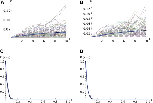
Comparison of analytic predictions with the simulation results for the idealized model described in the text. (A and B) Thin lines show xi for i = 0 to n = 10 for each replicate in which A was not lost before population 10. The thick black line shows the average of the 100 replicates and the thick blue line shows the expectation based on the analytic theory. (C and D) Probability that an allele reaches a frequency y in the final population when the range expansion is complete. In A–D, k = 100 and one copy of the mutant was present in the propagule founding population 1. In A and C, s1 = s2 = 0; in B and D, s1 = 0.005 and s2 = 0.01.
Realistic Model: Finite Population Size and Migration
To create a more realistic model, we assume each propagule grows in one generation to size N (> k) and remains at that size for T generations before generating a propagule that colonizes the next site. We also allow for migration: each established population, including population 0, receives immigrants at a rate m per generation from each neighboring population. The migration among established populations continues until all sites are occupied and the process is stopped. We are concerned with weak migration only and ignore the effect of migration on population growth and population size.
The composite parameter ke includes the effects of two opposing forces. Both the founder effect and the period of random mating after the population is founded increase the importance of genetic drift and hence reduce ke. Immigration from the neighboring population—there is only one for the population most recently founded—reduces the variance in allele frequency and hence increases ke. Whether ke is larger or smaller than k depends on the balance reached. A little algebra shows that if m 1, N 1, and T 2N, then if , independently of T.
Simulation Test of Realistic Model
We simulated the realistic model of range expansion described above. Each replicate begins with the frequency of A set to the specified initial frequency, x0. Then one cycle of colonization results in a frequency x1 in population 1. A cycle consists of the sampling of gametes to form a propagule; selection in the propagule; creation of population 1; and then T generations of migration, selection, and genetic drift in populations 0 and 1. The details of one cycle are described below. If x1 > 0, the next cycle begins with the formation of the propagule that will establish population 2. Cycles continue until either A is lost or all n populations are established. If xn ≥ 1/(2N), A survived the range expansion and the set of frequencies , the allele frequency trajectory, was retained for further analysis. This process was continued until a specified number of replicates in which A survived was obtained. The probability of survival was estimated to be the ratio of the number of replicates in which A survived to the total number of replicates run.
To compare the simulation results from the realistic model with the Wright–Fisher model, we used the analytic theory described above with k replaced by the integer nearest ke (Equation 9) and s1 and s2 by Ts1 and Ts2. The restriction to integer values of k is necessary because the Markov chain has to have an integer number of states.
Figure 2 shows two examples of the fit of the predictions of the Wright–Fisher model to the simulation results of the realistic model without migration. Figure 2, A–C, shows the results for a neutral allele and Figure 2, D–F, shows the results for a deleterious recessive allele (s1 = 0, s2 = 0.03). Figure 2, A and D, compares the probability that A reaches a specified frequency. Figure 2, B and E, compares the average frequencies, using the same format as Figure 1. Figure 2, C and F, compares the variances among replicates. These results are typical for other data sets. Without migration, the fit of the analytic predictions to the simulations is quite good for neutral and recessive deleterious alleles, at least for ks2 < 2. The predicted variances among replicates do not fit as well as the predicted averages, which is not surprising given that second moments are more variable than first moments. For selected alleles, the predicted tends to be slightly larger than the simulated values and the predicted tends to be slightly larger than the simulated values. Those tendencies are more pronounced for alleles with an additive deleterious effect on relative fitness (s2 = 2s1), particularly if ks2 > 1, which is large enough that such deleterious alleles would have little chance of increasing to high frequency. The extent to which all three predicted quantities fit the simulations is roughly similar.
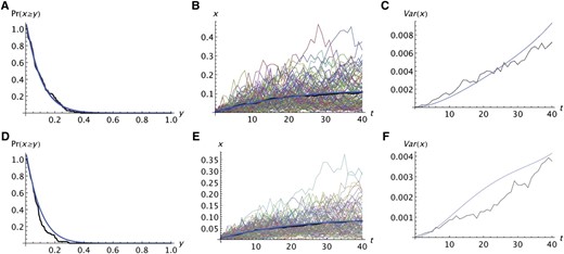
Comparison of analytic predictions of the Wright–Fisher model with the simulation result for the realistic model with no migration. The format is the same as in Figure 1. The analytic predictions were obtained by replacing k by the integer nearest ke and s1 and s2 by Ts1 and Ts2. In A–F, k = 100, N = 10,000, T = 5, and one copy of the mutant was present in the propagule founding population 1. The averages are over 100 replicate simulations. In A–C, s1 = s2 = 0; in D–F, s2 = 0.3 and s1 = 0 (recessive deleterious alleles).
With migration, the fit of the predictions to the simulations is not quite as good. Four examples are shown in Figure 3. Only the results for the average frequency are presented. With migration but no selection (Figure 3A), the analytic prediction tends to be slightly less than the average of the simulations. That tendency is also seen when there is migration and selection (Figure 3, B–D). Even when the number of colonization events is large enough that A is fixed in some of the replicates (Figure 3D), the predicted average frequency does not deviate by much from the analytic prediction.
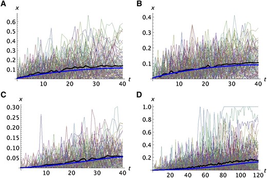
Comparison of analytic predictions with the simulation results for a model with finite population size and migration. The format is the same as in Figure 1, B and E. In A–D, k = 100, N = 1000, m = 0.04, and one copy of the mutant was present in the propagule founding population 1. In A, s2 = s1 = 0 (neutral); in B, s2 = 0.02 and s1 = 0 (recessive deleterious); in C, s2 = 0.02 and s1 = 0.01 (additive deleterious); in D, s2 = 0.01 and s1 = 0.005 (additive deleterious).
After the range expansion is complete, continuing migration will tend to smooth patterns created by the range expansion and continuing selection will cause the frequencies of deleterious alleles to gradually decay. Once the last population is colonized, our approximations for the expansion phase no longer apply. Subsequent evolution will be governed by the effective population sizes and selection intensities in each population. If the populations are large and selection is relatively strong, the decay will roughly follow the deterministic theory of selection and migration until allele frequencies become quite small. One example is presented in Figure 4.
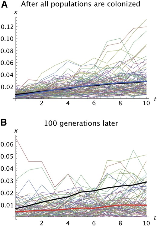
Illustration of the effects of continued evolution after all population are colonized. k = 100, N = 1000, T = 5, s2 = 0.01, s1 = 0.005, and m = 0.05. (A) Trajectories for 100 replicates immediately after the last population is colonized. The format is the same as in Figure 1, A and B. The prediction of the analytic model is shown in A by the thick blue line. The average of the 100 replicates immediately after all populations are colonized is shown by the thick black line in A and B. (B) The same set of trajectories 100 generations later. The thick red line shows the averages after 100 generations. Note the difference in the vertical scale in A and B.
The analytic approximation also provides an estimate of the probability that an allele will not be lost during the range expansion. Table 1 shows that the predicted and actual probabilities for the six cases shown in Figures 2 and 3 are in reasonable agreement, although the predictions tend to be larger than the simulated values.
Predicted and actual probabilities that an allele initially present in one copy in the propagule founding population 1 will be present in population n
| Predicted | Actual | |
|---|---|---|
| Figure 2, A–C | 0.048 | 0.043 |
| Figure 2, D–F | 0.047 | 0.038 |
| Figure 3A | 0.034 | 0.048 |
| Figure 3B | 0.047 | 0.031 |
| Figure 3C | 0.039 | 0.007 |
| Figure 3D | 0.013 | 0.0012 |
| Predicted | Actual | |
|---|---|---|
| Figure 2, A–C | 0.048 | 0.043 |
| Figure 2, D–F | 0.047 | 0.038 |
| Figure 3A | 0.034 | 0.048 |
| Figure 3B | 0.047 | 0.031 |
| Figure 3C | 0.039 | 0.007 |
| Figure 3D | 0.013 | 0.0012 |
| Predicted | Actual | |
|---|---|---|
| Figure 2, A–C | 0.048 | 0.043 |
| Figure 2, D–F | 0.047 | 0.038 |
| Figure 3A | 0.034 | 0.048 |
| Figure 3B | 0.047 | 0.031 |
| Figure 3C | 0.039 | 0.007 |
| Figure 3D | 0.013 | 0.0012 |
| Predicted | Actual | |
|---|---|---|
| Figure 2, A–C | 0.048 | 0.043 |
| Figure 2, D–F | 0.047 | 0.038 |
| Figure 3A | 0.034 | 0.048 |
| Figure 3B | 0.047 | 0.031 |
| Figure 3C | 0.039 | 0.007 |
| Figure 3D | 0.013 | 0.0012 |
We can explore further the probability that A will not be lost during the range expansion. Deleterious alleles of additive effect are lost quickly but deleterious recessive alleles have a substantial probability of not being lost even if their ultimate probability of fixation is low. Figure 5 shows some typical results for deleterious alleles. The probability that an allele survives is much lower for an allele of additive effect than for one that has a recessive effect.
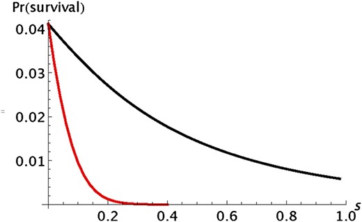
Illustration of the difference between alleles with an additive (red line) and a recessive (black line) effect on fitness. Pr(survival) is the probability that an allele initially present in one copy in population 0 is still present in population n. For both curves, k = n = 50 and s2 = s. For additive selection, s1 = s/2 and for recessive selection, s1 = 0. The results were obtained by iterating the transition matrix of the Markov chain.
The similarity of the model of range expansion and a model of a single population leads to a simple prediction about the loss in heterozygosity during a range expansion. The heterozygosity of neutral loci will be reduced by a factor of in each successive population.
Continuously Distributed Populations
Our results are based on a model in which populations are discrete. Much of the interest in range expansion comes from human and other populations that are continuously distributed in space. The relationship between continuous and discrete population models is not simple. As Felsenstein (1975) first noted, it is difficult to formulate a consistent model of a finite population that is continuously distributed in space and that maintains a uniform population density. The reason is that the assumption of uniform density is not compatible with the assumption that individuals reproduce independently of one another (Sawyer 1976). The usual resolution of this problem is to approximate a continuous model by a sequence of discrete models (Nagylaki 1978a,b).
We can relate the parameters of a discrete-population model to those of a model of a continuously distributed population as follows. A continuous-population model at equilibrium is characterized by the population density (ρ), the root-mean-square dispersal distance (σ), and the total length of the habitat (L). The correspondence between discrete and continuous models in a one-dimensional habitat is well established for populations at equilibrium. If L is large enough that end effects do not dominate, the heterozygosity and decrease in the probability of identity-by-descent of neutral alleles in a continuous-population model are the same as in a discrete-population model when and , where l = L/n is the distance between adjacent populations (Malécot 1975). Therefore, to recover the parameters of the discrete-population model, for which we have an analytic approximation, , , and , where l is not yet specified.
To determine l, we assume that new individuals beyond the leading edge of the population are randomly sampled from k individuals at or near the leading edge. Range expansion occurs as new individuals appear in such a way that their average density is ρ. This assumption fits the observation of Hallatschek et al. (2007) who found that, in an experimental study of range expansion in Escherichia coli, colonists appeared to come predominantly from the small number of cells at the expanding edge of the population. In a continuously distributed population expanding at a uniform rate, there is no delay corresponding to the T generations allowed for in the discrete-population model. Hence T can be set to 1. In the continuous model, a habitat of length L is colonized in total time τ, which corresponds to n generations in the discrete-population model. Therefore, n = τ, which we have already determined to be L/l, and consequently l = L/τ.
Discussion and Conclusions
We show that range expansion in a one-dimensional habitat is similar in some ways to random mating in a single population. The succession of colonization events during range expansion creates a spatial sequence of allele frequencies that is analogous to the time sequence of allele frequencies in a single population. This is true in an idealized model of range expansion and is approximately true in a more realistic model that allows for some delay before the next colonization event and for weak gene flow among established populations. The similarity of the two models allows the theory of random mating to be adapted to make analytic predictions about the consequences of range expansions. There is a strong stochastic component to the process that makes prediction of individual allele frequency trajectories difficult, but the average trajectory and the extent of variation among them are well predicted by the analytic theory.
Although our simulation results are for a model of instantaneous population growth, our analytic theory makes clear that the effective number of colonists, ke, depends partly on the net effect of genetic drift between successive colonization events and hence can be defined for other models of population growth including the logistic model.
Previous work on the effects of surfing has emphasized that surfing can drive some initially rare alleles to high frequency (Travis et al. 2007; Hallatschek and Nelson 2010; Hallatschek 2011). The probability that an initially rare allele is fixed in a randomly mating population can be calculated from a diffusion approximation (Kimura 1962). Roughly speaking, deleterious alleles have a significant probability of being fixed by genetic drift if Ns ≤ 1, where N is the population size and s is the selection coefficient. In the context of range expansions, our approximate theory tells us that the probability that an initially rare allele is driven to fixation during a range expansion depends on the product kese, where ke is the effective propagule size (Equation 9) and se is the effective selection coefficient (Equations 10 and 11). This provides an approximate way to determine whether a deleterious allele has a significant probability of surfing to a high frequency. It implies that expanding populations could accumulate deleterious mutations at a faster rate than equilibrium populations, which could potentially explain the observed excess of deleterious alleles in Europeans (Lohmueller et al. 2008) or the collapse of some invading species (Cooling et al. 2011).
Clines in allele frequency are often attributed to geographic variation in selection intensities. In humans, clines in the frequencies of alleles that cause monogenic diseases are observed and sometimes attributed to unknown environmental conditions (Novembre and Di Rienzo 2009). For example, the Δ508 allele of CFTR associated with cystic fibrosis (Bertranpetit and Calafell 1996) and the C282Y mutation of hemochromatosis (Lucotte and Dieterlen 2003) have a higher frequency in northern than in southern Europe. Our results show that such clines could be created by range expansion in the absence of any geographic variation in selection intensity. Several authors (Handley et al. 2007; DeGiorgio et al. 2009; Hunley et al. 2009) have emphasized the importance of nonequilibrium processes in structuring human and other populations and the need to consider neutral explanations for apparently adaptive patterns.
Our theory also predicts the slope of a gradient on heterozygosity that results from range expansion in a one-dimensional habitat and can be recast in terms of a continuous habitat. This correspondence allows us to obtain a rough estimate of the effective propagule size on the basis of the data of Ramachandran et al. (2005).
Acknowledgements
M.S. was partially supported by a grant from the U.S. National Institutes of Health, R01-GM40282. L.E. was partially supported by a Swiss National Science Foundation grant, 3100A0-126074.
Literature Cited
Appendix A
Derivation of Effective Number of Founders
In this derivation, we have not included the effect of migration from the newly founded population back into the source of the colonists. This back migration would change x0 slightly. We justify ignoring this change because it is of the same order of magnitude as the migration rate, m, and hence will modify the effect of immigration on the variance in the newly founded population by a term that is only of order m2.
Appendix B
Derivation of the Effective Selection Coefficients
Footnotes
Communicating editor: W. Stephan
