Bayesian Detection of Expression Quantitative Trait Loci Hot Spots

Abstract

THE current focus of biological research has turned to high-throughput genomics, which encompasses large-scale data generation and a variety of integrated approaches that combine two or more -omics of data sets. An important example of integrative genomics analysis is the investigation of the genetic regulation of transcription, also called expression quantitative trait locus (eQTL) or “genetical genomics” studies (Cookson et al. 2009; Majewski and Pastinen 2011). A typical eQTL analysis follows a natural structure of parallel regressions between the large set of q responses (i.e., expression phenotypes), and that of p explanatory variables (i.e., genetic markers, often single nucleotide polymorphism, SNPs), where p is typically much larger than the number of observations n.

From a statistical point of view, the size and the complex multidimensional structure of eQTL data sets pose a significant challenge. Not only does one wish to detect the set of important genetic control points for each response (expression phenotype), including cis- and trans-acting control for the same transcript, but, ideally, one would wish to exploit the dependence between multiple expression phenotypes. This will facilitate the discovery of key regulatory markers, so-called hotspots (Breitling et al. 2008), i.e., genetic loci or single polymorphisms that influence a large number of transcripts. Identification of hotspots can inform on network and pathways, which are likely to be controlled by major regulators or transcription factors (Yvert et al. 2003; Wu et al. 2008). Most importantly, there is mounting evidence that common diseases may be caused (or modulated) by changes at a few regulatory control points of the system (i.e., hotspots), which can cause perturbations with large phenotypic effects (Chen et al. 2008; Schadt 2009).

In this article, we set out to perform hotspot and eQTL detection in an efficient manner, which exploits fully the multidimensional dependencies within the genome-wide gene expression and genetic data sets. We build upon our previous work (Bottolo and Richardson 2010), where we implemented Bayesian sparse multivariate regression for continuous response to search over the possible subsets of predictors in the large 2^p model space. For each expression phenotype, this corresponds to carrying out multipoint mapping within an inference framework, Bayesian variable selection (BVS), where model uncertainty is fully integrated. Here, we propose a novel structure for linking parallel multivariate regressions that borrows information in a hierarchical manner between the phenotypes to highlight the hotspots. To be precise, we propose a new multiplicative decomposition of the joint matrix of selection probabilities ω_kj that link marker j to phenotype k and demonstrate in a simulation study that this hierarchical structure and its Bayesian implementation (hierarchical evolutionary stochastic search or HESS algorithm) possess good characteristics in terms of sensitivity and specificity, outperforming current methods for hotspot and eQTL detection. Finally, we show the applicability of our method in two real-case eQTL studies, including animal models and human data. Our approach is broadly applicable and extendable to other high-dimensional genomic data sets and represents a first step toward a more reliable identification of functional eQTL hotspots and the underlying causal regulators.

Analysis models for eQTL data are linked to two strands of work: (i) methods for multiple mapping of QTL, where a single continuous response, referred to as a “trait,” is linked to DNA variation at multiple genetic loci by using a multivariate regression approach, and (ii) models that exploit the pattern of dependence between the sets of responses associated with a predictor (i.e., genetic marker). There is a vast literature on multi-mapping QTL (see the review by Yi and Shriner 2008); some of the models have been extended to the analysis of a small number of traits simultaneously (Banerjee et al. 2008; Xu et al. 2008). Several styles of approaches have been adopted ranging from adaptive shrinkage (Yi and Xu 2008; Sun et al. 2010) to variable selection within a composite model space framework that sets an upper bound on the number of effects (Yi et al. 2007). Most of the implemented algorithms sample the regression coefficients via Gibbs sampling. However, these have not been used with a substantial set of markers in the “large p small n” paradigm, but mostly in case of candidate genes or in small experimental cross-animal studies. To face the challenges typical of larger eQTL studies, we have chosen to build our multi-mapping model using a recently developed Bayesian sparse regression approach (Bottolo and Richardson 2010). In this approach, subset selection is implemented in an efficient way for vast (potentially multi-modes) model space by integrating out the regression coefficients and by using a purposely designed MCMC variable selection algorithm that enhances the model search with ideas and moves inspired by evolutionary Monte Carlo algorithms.

The first eQTL modeling approach that explicitly set out to borrow information from all the transcripts was proposed by Kendziorski et al. (2006). In the mixture over markers (MOM) method, each response (expression phenotype) y_k, 1 ≤ k ≤ q, is potentially linked to the marker j with probability p_j or not linked to any marker with probability p₀. All responses linked to the marker j are then assumed to follow a common distribution f_j(⋅), borrowing strength from each other, while those of nonmapping transcripts have distribution f₀. Inspired by models that have been successful for finding differential expression, the marginal distribution of the data for each response y_k is thus given by a mixture model: $p0f0(yk)+∑j=1ppjfj(yk)$⁠. A basic assumption of the MOM model is that a response is associated with at most one predictor. For good identifiability of the mixture, MOM requires a sufficient number of transcripts to be associated with the markers. The authors use the EM algorithm to fit the mixture model and estimate the posterior probability of mapping nowhere or to any of the p locations. By combining information across the responses, MOM is more powerful and can achieve a better control of false discovery rates (FDR) by thresholding the posterior probabilities than pure univariate differential expression methods testing each transcript-marker pair. But as originally developed, it is not fully multivariate as it does not account for multiple effects of several markers on each expression trait.

The high dimensionality of both gene expression and marker space has been alternatively addressed through the use of data reduction methods. In particular, Chun and Keleş (2009) have proposed implementing sparse partial least-squares regression (M-SPLS eQTL) on preclustered group of transcripts. M-SPLS selects markers associated with each transcript cluster by evaluating the loadings on a set of latent components. As the dimension of each cluster is moderate, SPLS implements a multivariate formulation that takes into account the correlation between the transcripts in the same cluster. Sparsity of the latent direction vectors is achieved by imposing a combination of L₁ and L₂ penalties, similar to the elastic net. The tuning parameters K and η controlling the number of latent components and the convexity of the penalized likelihood are tuned together by cross-validation. The output of this method is the set of the regression coefficients of the markers belonging to the latent vectors that are significantly associated with a subset of transcripts, selected by bootstrap confidence interval.

Jia and Xu’s linked regression set-up and fully Bayesian formulation is a natural starting point for eQTL detection, which shares common features with our approach. Here, we present a novel model structure and state of the art implementation based upon evolutionary Monte Carlo. We report the results of a simulation study comparing our HESS method to BAYES (Jia and Xu 2007), as well as to two alternative approaches: MOM (Kendziorski et al. 2006) and M-SPLS (Chun and Keleş 2009). Finally, we show the application of our method to two diverse genomic experiments in mouse and human genetic contexts.

Theory and Methods

Hierarchical related sparse regression

The description of the joint likelihood as the product of q regression equations is similar to the one proposed by Jia and Xu (2007). However, one important difference is the assignment in (2) of a regression specific error variance $σk2$⁠, allowing for transcript-related residual heterogeneity and making our formulation more flexible. A more general model, seemingly unrelated regressions (SUR) introduces additional dependence between the responses Y through the noise ε_k, modeling the correlation between the residuals of different responses (Banerjee et al. 2008). However, it becomes computational unfeasible when the size of q is large, which is typical in eQTL experiments.

Prior set-up

The hierarchical structure on the regression coefficients is completed by specifying a hyper-prior on the scaling coefficient τ, p(τ). We adopt the Zellner–Siow priors structure for the regression coefficients that can be thought as a scale mixture of g-priors and an inverse-gamma prior on τ, p(τ) = Inv Ga(1/2, n/2) with heavier tails than the normal distribution, $p(βk|γk,σk2)=Cauchy(0,nσk2(XγkTXγk)−1)$⁠. In general it has been observed (Bottolo and Richardson 2010) that data adaptivity of the degree of shrinkage conforms better to different variable selection scenarios than assuming standard fixed values (which can be easily implemented by using a point mass prior for τ). Since the level of shrinkage can influence the results of the variable selection procedure, in our model we force all the q regression equations to share the same common τ, linking the regression equations hierarchically through the variance of their nonzero coefficients.

The prior specification is concluded by assigning a Bernoulli prior on the latent binary value γ_kj, p(γ_kj|ω_kj) = Bernoulli (ω_kj). The prior chosen for ω_kj is of paramount importance in BVS since it controls the level of sparsity, i.e., the association with a parsimonious set of important predictors. For a given response this task can be accomplished by specifying a common small-selection probability for all p predictors, ω_kj = ω_k and giving p(ω_k) = Beta(a_k, b_k) (Bottolo and Richardson 2010). Inducing sparsity when all the responses are jointly considered is harder because further constraints are desirable. eQTL surveys (Cookson et al. 2009) suggest that only a fraction of expression traits are under genetic regulation and the number of their control points is usually small. This can be modeled by assigning a different probability for each marker ω_kj = ω_j with an hyper-prior on ω_j. This solution, first proposed by Jia and Xu (2007) with the conjugate prior p(ω_j) = Dirichlet(d_1j, d_2j), assumes that this selection probability is the same for all the responses. However, whatever the sensible choice of the hyperparameters d_1j and d_2j,  d_1j, d_2j = 1 or d_1j, d_2j = 0.5, the posterior density greatly depends on the ratio between the number of transcripts associated to the marker j, q_j, and the total number the transcripts in the eQTL experiment, q, since E(ω_j|Y) = (q_j + d_1j)/(q + d_1j + d_2j), where q_j = # {j: γ_kj = 1}. In such formulation, the results are thus clearly influenced by the number of responses analyzed and sparsity of each kth regression cannot be controlled in the prior specification adopted for ω_kj of γ_kj.

We conclude this section by describing the choice of the hyperparameters for ω_k and ρ_j. Since by construction ω_k ⊥ ρ_j, E(ω_jk) = E(ω_k)E(ρ_j). If we assume c = d, the hotspot propensity does not change the a priori row marginal expectation, E(ω_jk) = E(ω_k). However, it inflates the a priori row marginal variance Var(ω_jk) > Var(ω_k), with Var(ω_jk) = Var(ω_k)(1 + d⁻¹) + d⁻¹E²(ω_k). For the specification of the hyperparameters a_k and b_k, we use the Beta-binomial approach illustrated in Kohn et al. (2001), after marginalizing over the column effect in (5). The two hyperparameters can be worked out once E(p_γk) and Var(p_γk), the expected number and the variance of the number of genetic control points for each response, are specified.

Posterior inference

Sampling Γ is extremely challenging since complex dependence structures in the X create well-known problems of multimodality of the model space even for a single regression equation. Here the computational challenge is higher since we are aiming to explore a huge model space of dimension (2^p)^q. For this reason vanilla MCMC (MC³, Gibbs sampler, simple dimension changing moves) cannot guarantee a reliable exploration of the model space in a limited number of iterations. In this article we use a sampling scheme introduced by Bottolo and Richardson (2010), evolutionary stochastic search (ESS) as a building block for our new algorithm HESS. For each response, HESS relies on running multiple chains with different “temperature” in parallel, which exchange information about the set of covariates that are selected in each chain. Since chains with higher temperatures flatten the posterior density, global moves (between chains) allow the algorithm to jump from one local mode to another. Local moves (within chains) permit the fine exploration of alternative models, resulting in a combined algorithm that ensures that the chains mix efficiently and do not become trapped in local modes. Specific modifications of ESS were introduced to comply with the structure of ω_kj, which are sampled with the decomposition (5) rather than integrating them out as in ESS. This requires some modifications in the local moves (details in Supporting Information, File S1, Section S.2.2.)

For sampling the selection probability matrix Ω, we implemented a Metropolis-within-Gibbs algorithm for each element of the row effect ω = (ω₁, …, ω_q)^T and column effects ρ = (ρ₁, …, ρ_q)^T, rejecting proposed values outside the range [0, 1]. However, since the dimension of ω and ρ is very large, tuning the proposal for each element of the two vectors is prohibitive. To make HESS fully automatic, we use the adaptive MCMC scheme proposed by Roberts and Rosenthal (2009), where the variance of the proposal density is tuned during the MCMC to reach a specified acceptance rate. To satisfy the asymptotic convergence of the adaptive MCMC scheme, mild conditions are imposed (details in File S1, Section S.2.3).

If not fixed, the scaling coefficient τ, which is common for all the q regression equations and all the L chains, is sampled using a Metropolis-within-Gibbs algorithm with random walk proposal and fixed proposal variance (details in File S1, Section S.2.4).

Finally, we describe a complete sweep of our algorithm. We assume that the design matrix is fully known. If missing values are present, these can be imputed in a preprocessing imputation step (for instance using the fill.geno function from the qtl R package for genetic crosses (Broman and Sen 2009) or FastPhase (Scheet and Stephens 2006) for human data). Without loss of generality, we assume that the responses and the design matrix have both been centered. The same notation is used when τ is fixed or given a prior distribution. For simplicity of notation we do not index variables by the chain index, but we emphasize that the description below applies to each chain:

• Given Ω and τ we update γ_k, according to the ESS procedure, using global and local moves. During the burn-in, we sample the latent binary vector γ_k for each k to tune the regression specific temperature ladder (details in File S1, Section S.2.5). After the burn-in, at each sweep, we select at random without replacement a fraction φ of the regressions where to update γ_k.

• Given Γ and τ, we sample ω and ρ with a random walk Metropolis with adaptive proposals.

• Given Γ and Ω, we sample τ with a random walk Metropolis with a fixed proposal. To balance the number of updates of the latent binary values γ_kj with those of the scaling coefficient, at each sweep, the number of times we sample τ is proportional to q × p × L.

The Matlab implementation of the HESS algorithm is available upon request from the authors.

Postprocessing analysis

In this section we present some of the postprocessing operations required to extract useful information from the rich output of our model. We stress that, while here for simplicity we are not using the output of the heated chains, following Gramacy et al. (2010), posterior inference could also be carried out using the information contained in all the chains.

Results

Simulation studies

We carried out a simulation study to compare our algorithm with recently proposed multiple response models: MOM (Kendziorski et al. 2006), BAYES (Jia and Xu 2007), and M-SPLS (Chun and Keleş 2009).

To create more realistic examples, we decided not to simulate the X matrix, but to use real human-phased genotype data spanning 500 kb, region ENm014 (chromosome 7: 126,368,183–126,865,324 bp), from the Yoruba population used in the HapMap project (Altshuler et al. 2005) as the design matrix. After removing redundant variables, the set of SNPs is reduced to P = 498, with n = 120, giving a 120 × 498 X matrix. As noted by Chun and Keleş (2009), high correlations between markers might affect the performance of variable selection procedures that do not explicitly consider such a grouping structure. The benefit of using real human data are to test competing algorithms when the pattern of correlation, i.e., linkage disequilibrium (LD), is complex and blocks of LD are not artificial, but they derive naturally from genetic forces, with a slow decay of the level of correlation between SNPs (see Figure S1).

In the simulated examples, we carefully select the SNPs that represent the hotspots (Figure S1): (i) all hotspots are inside blocks of correlated variables; (ii) the first four SNPs are weakly dependent (r² < 0.1); and (iii) the remaining two SNPs are correlated with each other (r² = 0.46) and also linked to one of the previous simulated hotspots (r² = 0.52 and r² = 0.44, respectively), creating a potential masking effect difficult to detect. Apart from the hotspots, no other SNPs are used to simulate transcript–SNP associations. We simulated four cases:

• SIM1: In this example we simulated q = 100 transcripts from the selected six hotspots, with some transcripts predicted by multiple correlated markers (polygenic control): for instance transcripts 17–20 are regulated by three SNPs at the same time (see Figure S2). Altogether we simulated 94 transcript–SNP associations in 50 distinct transcripts. The effects were simulated from a normal density with smaller variance than in Jia and Xu (2007), β_kj ∼ N(0,0.3²)with ε_k ∼ N(0, 0.1²I_n) to mimic the smaller signal-to-noise ratio expected in genetically heterogeneous human data.

• SIM2: As in the previous example, we simulated 100 responses, but there are only three hotspots with the same simulated association as before, leading to 64 transcript–SNP associations in 30 distinct transcripts. Moreover we created potential false-positive associations by simulating transcripts 81–90 and 91–100 using a linear transformation of transcript 20 with a mild negative correlation (in the interval [−0.5, −0.4]) and of transcript 80 with a strong positive correlation (in the interval [0.8, 0.9]), respectively. Since we create false-positive associations, the scenario will inform on how different algorithms behave when correlations among some transcripts are not due to SNPs.

• SIM3: This simulation set-up is identical to the first scenario for the first 100 responses, but we increase the number of simulated responses to q = 1,000, simulating the further 900 transcripts from the noise.

• SIM4: This is the same as the second simulated data set for the first 100 responses, with additional 900 responses simulated from the noise, giving altogether q = 1000 responses.

We discuss here the hyperparameters set-up. Since a priori, in addition to a large effect of a SNP that is located close to the transcript (cis-eQTL), we expect only a few additional control points associated with the variation of gene expression (typically trans-eQTL); in HESS we set E(p_γk) = 2 and Var(p_γk) = 2, meaning the prior model size for each transcript response is likely to range from 0 to 6 (Petretto et al. 2010). Following Kohn et al. (2001), we fixed a_σ = 10⁻¹⁰ and b_σ = 10⁻³, giving rise to a noninformative prior on the error variance. We run the HESS algorithm for 6000 sweeps with 1000 as burn-in with three chains and ϕ = 1/4. Computational time is similar for the first two simulated examples, 6 hr, and 10 times greater for the last two simulated scenarios on a Intel Xeon CPU at 3.33 GHz with 24 Gb RAM.

We run BAYES for 15,000 sweeps with 5000 as burn-in, recording sampled values every 5 sweeps. The variance δ of the spike component 1 is set 10⁻⁴, which is 100 times lower than the noise variance. Since the code available from the authors was written in SAS/IML, we recoded their Gibbs sampler in Matlab. We used the default parameters for MOM, while in M-SPLS the two tuning parameters are obtained through cross-validation selected in the interval K = 1,…, 10 and η = 0.01, …, 0.99. Each simulated example was replicated 25 times and we run the four algorithms on each replicate.

Power to detect hotspots:

The identification of the hotspots is of primary interest for all the algorithms we are comparing. In HESS using the tail posterior probability Pr(ρ_j >1|Y), we can rank the predictors according to their propensity to be a hotspot, while in BAYES the posterior mean of the common latent probability ω_j,  E(ω_j|Y) is utilized to prioritize important markers. In MOM the strength for a predictor to be a hotspot is not directly available but, as suggested by the authors, given a marker, it can be obtained by taking a suitable quantile of the transcript–marker associations distribution across responses. We use their R function get.hotspots recording the average of the distribution for each predictor. M-SPLS, after cross-validation, provides a list of latent components that predicts most of the variability of Y. While this group cannot be interpreted directly as the list of hotspots, we use it to test the existing overlap between the simulated hotspots and the latent components. Finally, differently from the analyses presented in Jia and Xu (2007) and Chun and Keleş (2009), in the HESS power calculation, we simply rank the evidence for being a hotspot provided by each algorithm across the 25 replicates. Therefore we are not using any method-specific procedure to call a hotspot, based for instance on FDR considerations, that could influence the comparison results.

Figure 1 shows the ROC curves for the four algorithms considered. HESS (blue lines) outperforms all the other methods with sizeable power on the simulated examples. It is not significantly affected by the dimension of the eQTL experiment (top, q = 100; bottom, q = 1000). This is somehow expected since the hotspot propensity does not depend directly on the number of transcripts analyzed (see File S1, section S.2.3). Spurious correlations among transcripts not due to SNPs (right) have a negligible effect on the HESS power, showing robust properties of our algorithm in detecting hotspots under different scenarios.

Figure 1

Open in new tabDownload slide

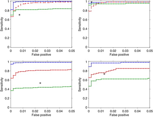
ROC curves for hotspots detection using HESS (blue line), MOM (red line), BAYES (green line), and M-SPLS (black star) in the four simulated scenarios (Figure S2). From top to bottom, left to right: SIM1, q = 100 and six hotspots; SIM2, q = 100 and three hotspots; SIM3, q = 1000 and six hotspots; SIM4, q = 1000 and three hotspots. For M-SPLS, type I error and power were calculated conditionally on the list of latent vector components. (Top) MOM is indicated by a red dashed line to highlight that it is not designed in the cases when the number of markers is larger than the number of traits.

The other methods show good properties when q = 100, but their power degrades sensibly when q = 1000. This is expected for BAYES (green lines) since E(ω_j|Y) is affected by q, while the performance of MOM (red lines) is more stable. MOM (red dashed lines) shows good power in the simulated examples even when the number of markers is larger than the number of traits, a situation that MOM is not designed for (top). Finally M-SPLS has greater power than BAYES, but it is outperformed by both HESS and MOM in the more sparse scenarios (bottom). Looking more closely at the list of latent vectors identified by M-SPLS (data not shown), we noted that the simulated hotspots at SNP 362 and 466 that are linked to SNP 239 were rarely selected (false negative) in both SIM1 and SIM3. On the contrary, SNP 75 is very often included (false positive) in the list of latent vectors in all the scenarios. This might reflect the high correlation between SNP 362 and 466 with SNP 239, as well as the strong dependency between SNP 75 and 30 where we simulated a hotspot. This suggests that M-SPLS has limited efficiency in the presence of complex correlation patterns in the design matrix. In Figure S3, Figure S4, Figure S5, and Figure S6, interested readers can find the visual representation of the signals detected by each algorithm and averaged across the 25 replicates.

Power to detect transcript-marker associations:

Figure 2 shows the ROC curves of the transcript–marker marginal associations detected by each method. Also in this case, to perform the power calculation, we are not using any method-specific way to declare a significant association, since we simply record the output from each algorithm and rank it across the 25 replicates. In particular we use the marginal probability of inclusion p(γ_kj = 1|y_k) (8) for HESS; the posterior frequency $γ¯kj=Σs=1Sγkj(s)/S$ for BAYES, where $γkj(s)$ is the value recorded at iteration s; the transcript–marker association provided the MOM object momObj; and finally the associations selected by bootstrap confidence interval at different type I error levels (α = 10⁻⁴, 10⁻³, 10⁻², 0.05) for M-SPLS.

Figure 2

Open in new tabDownload slide

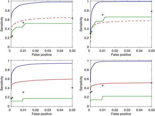
ROC curves for transcript–marker associations using HESS (blue line), MOM (red line), BAYES (green line), and M-SPLS (black star) in the four simulated scenarios (Figure S2). From top to bottom, left to right: SIM1, q = 100 and six hotspots; SIM2, q = 100 and three hotspots; SIM3, q = 1000 and six hotspots; SIM4, q = 1000 and three hotspots. For M-SPLS, power is calculated conditionally on the list of transcript–marker associations selected by bootstrap confidence interval at a fixed type I error (α = 10⁻⁴, 10⁻³, 10⁻², 0.05). In the top, MOM is indicated by a red dashed line to highlight that it is not designed in the cases when the number of markers is larger than the number of traits.

For transcript–marker association detection, we find that HESS has higher power than that of the other methods in all the simulated scenarios. As expected when more responses are included, the power decreases slightly (bottom), while spurious associations due to the correlation between transcripts do not seem to affect the ability of HESS to distinguish between true and false signals (right). MOM is quite stable across scenarios, but it reaches only half of the power of HESS. BAYES and M-SPLS have similar behavior and their performance degrades when q = 1000. BAYES, in particular, has very low power since the shrinkage to the null effect, caused by common latent probabilityω_j, is particularly strong in SIM3 and SIM4.

The different power of the methods considered can be better understood by looking at Figure S3, Figure S4, Figure S5, and Figure S6, where, for each simulated example, we averaged the evidence of transcript–marker association across replicates. HESS is able to identify the correct simulated pattern, with very few false positives. When false-positive associations are simulated, for instance, in SIM3 and SIM4, HESS assigns on average lower posterior probability of inclusion than for the true positive ones (Figure S4 and Figure S6, top left). While MOM is able to identify the simulated hotspots, it finds it difficult to separate the true transcript–marker associations from the spurious ones (Figure S3, Figure S4, Figure S5, and Figure S6, bottom left). The main limitation of M-SPLS is the correct identification of the latent vectors when highly correlated predictors are considered (Figure S3, Figure S4, Figure S5, and Figure S6, top right). Finally BAYES is able to identify the simulated pattern when q = 100 (Figure S3 and Figure S4, bottom right), but it seems to be too conservative when the number of responses is large, q = 1000 (Figure S5 and Figure S6, bottom right). The higher false-negative rate in BAYES may depend on the poor efficiency of the MCMC sampler (which is based exclusively on the Gibbs sampling that is not able to jump between distant competing models) and on the spike and slab prior that is not integrated out. The latter influences the sampling of γ_kj since the latent binary vector depends on the regression coefficients (see Figure S7 for an illustration).

Real case studies

Here we present two applications of HESS to: (i) mouse gene expression data published in Lan et al. (2006) that is commonly used as a benchmark data set for detection of eQTL (Chun and Keleş 2009) and eQTL hotspots (Kendziorski et al. 2006; Jia and Xu 2007) and (ii) human monocytes expression data set recently analyzed for disease susceptibility by Zeller et al. (2010).

Mouse data set:

The mouse data set has been previously described in detail (Lan et al. 2006), and it consists of 45,265 probe sets the expression of which has been measured in the liver of 60 mice. Mice were collected from the F₂-ob/ob cross (B6 × BTBR) and genotype data were available for 145 microsatellite markers from 19 autosomal chromosomes. To make our analysis comparable with previously reported studies (Jia and Xu 2007; Chun and Keleş 2009), we focused on 1573 probe sets showing sizeable variation in gene expression in the mouse population (sample variance >0.12). Running HESS for 12,000 sweeps with 2000 as burn-in and the same choice of the hyperparameters described in the simulation studies, among the 145 markers 16 were identified with posterior tail probability >0.8, regulating a significant number of probe sets (Table S1). We report the genome location of the identified hotspots in Figure 3 and show transcript–marker associations in Figure 4. Since large hotspot propensity reveals that multiple traits are controlled by the same marker, we focused on biologically meaningful transcript–marker associations by using marginal probability of association >0.95 (corresponding to local FDR 5%, Ghosh et al. 2006). Six markers were found to control more than 5% of all analyzed probe sets as shown in Figure 3. While marker D15Mit63 was previously detected by BAYES and M-SPLS, three other major regulatory points were identified solely by our method: D13Mit91, D18Mit9, and D18Mit202, controlling 14.1, 10.6, and 9.7% of all analyzed probe sets, respectively (Table S2).

Figure 3

Open in new tabDownload slide

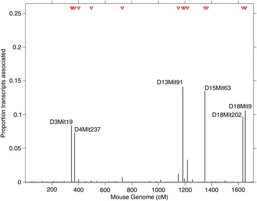
Proportion of transcripts associated with each marker in the mouse data example (n = 60, P = 145, and q = 1573). Transcript–marker association was declared at 5% local FDR with marginal probability of inclusion >0.95. The 16 red triangles indicate markers (two of them are overlapping and hence are not distinguishable) that have been identified as hotspots with tail posterior probability >0.8.

Figure 4

Open in new tabDownload slide

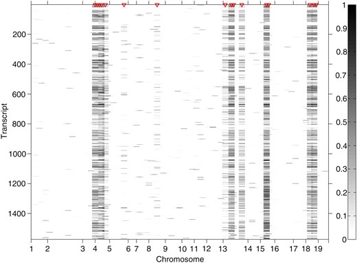
Heat map of the marginal probabilities of inclusion for each transcript–marker pair in the mouse data example (n = 60, P = 145, and q = 1573). The 16 red triangles indicate markers that have been identified as hotspots with tail posterior probability >0.8.

The regulatory hotspot at marker D13Mit91 is located within the Kif13a (kinesin family member 13A) gene, which is involved in intracellular protein transport and microtubule motor activity via direct interaction with the AP-1 adaptor complex (Nakagawa et al. 2000). This hotspot is associated with 222 probe sets, representing 190 distinct well-annotated genes, that are enriched for specific gene ontology (GO) terms, including “protein localization” (P = 4.2 × 10⁻⁶), “protein transport” (P = 5.7 × 10⁻⁶), and “establishment of protein localization” (P = 6.4 × 10⁻⁶). Hence, given its molecular function Kif13a is likely to be a candidate master regulator of the genes implicated with protein transport, and whose expression is associated with marker D13Mit91.

The other two newly identified markers, D18Mit9 and D18Mit202, are located on mouse chromosome 18. D18Mit9 resides within a known QTL (Hdlq30) involved in HDL cholesterol levels (Korstanje et al. 2004) whereas D18Mit202 resides within a known diabetes susceptibility/resistance locus (Idd21, insulin-dependent diabetes susceptibility 21) (Hall et al. 2003).

Human data set:

The human data set included 648 probe sets, representing 516 unique and well-annotated genes (Ensemble GRCh37), that were found to be coexpressed in monocytes, delineating a network driven by the IRF7 transcription factor in 1490 individuals from the Gutenberg Heart Study (GHS) (for details on the network analysis, see Heinig et al. (2010)). This IRF7-driven inflammatory network (IDIN) was also reconstructed in a distinct population cohort: 758 subjects from the Cardiogenics Study showing significant overlap with the network in GHS. The “core” of the network consisted of a small gene set (q = 17), including IRF7 and coregulated target genes, the expression of which was found to be trans-regulated by a locus on human chromosome 13q32 using MANOVA in Cardiogenics (Heinig et al. 2010). However, this trans-regulation was not found in the GHS study, using similar MANOVA analysis.

Here we take a new look and use HESS to analyze the larger IDIN with 648 probe sets in the GHS population (n = 1490 individuals) and the SNP set (P = 209) spanning 1 Mb on chromosome 13q32 (data available upon request from Stefan Blankenberg under the framework of a formalized collaboration via a Memorandum Transfer Agreement). While MOM and BAYES fail to detect any signal at this locus, using HESS we found two SNPs, rs9557207 and rs11616269, which are detected as hotspots for the IDIN expression with tail posterior probability 0.83 and 0.91, respectively (Figure 5). These SNPs are located 45.3 kb (rs9557207) and 25.1 kb (rs11616269) from SNP rs9585056, which previously showed significant trans-effect on the core gene set of the network in Cardiogenics (P = 5.0 × 10⁻³). This region was also associated with EBI2 expression (P = 2.2 × 10⁻⁸), the candidate gene at this locus, and with type I diabetes (T1D) (P = 7.0 × 10⁻¹⁰) (Heinig et al. 2010). For the two identified hotspots, we looked in detail at each transcript–marker association and compute their BF as given in (9). We observe that 26 and 13 transcripts show clear evidence of associations (BF > 10, Kass and Raftery 2007) in the two hotspots identified (Table S3) delineating the extent of regulatory effects. To further calibrate this evidence, we investigated BF for marker–transcript associations in a comparable simulated set-up, that of SIM3. Using the threshold BF > 10 would lead to declaring <5% false positive marker–transcript associations in the identified hotspots (data not shown). Note that most of these transcripts (80%) are found only in the network inferred in GHS and not with the Cardiogenics network, suggesting a complex pattern of regulatory effects around locus rs9585056 which is highlighted in a specific manner in each population. These population-specific regulatory effects could reflect differences in monocytes selection protocols between GHS and Cardiogenics (see Heinig et al. (2010) for details). However, the identification of hotspots at the 13q32 locus by HESS in GHS represents a significant replication of the findings previously reported, which reflects the increased power of HESS over alternative methods.

Figure 5

Open in new tabDownload slide

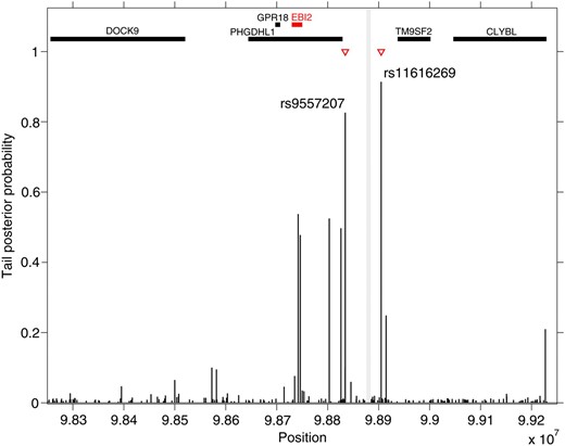
Tail posterior probability for each marker in the human data example (Gutenberg Heart Study, n = 1490, P = 209, and q = 648). Red triangles indicate markers that have been identified as hotspots with tail posterior probability >0.8. The vertical gray line highlights the physical position of annotated SNP rs9557217 and rs9585056 that were previously associated with IDIN network in the Cardiogenics Study cohort and EBI2 expression (Heinig et al. 2010). Thick horizontal bars on the top of the figure display physical position of genes in the 1-Mb region obtained from Ensemble database.

Discussion

We have presented a new hierarchical model and algorithm, HESS, for regression analysis of a large number of responses and predictors and have applied this to hotspot discovery in eQTL experiments. Simulating a variety of complex scenarios, we have demonstrated that our approach outperforms currently used algorithms. In particular, HESS shows increased power to detect hotspots when a large number of transcripts are jointly analyzed. This is due to the propensity measure ρ_j that we use, which quantifies the latent hotspot effect independently of the response dimensionality. One improvement of HESS over vanilla MCMC-based algorithms is in the search procedure that efficiently probes alternative models and assesses their importance, thus providing a reliable model space exploration (Bottolo and Richardson 2010). We have also illustrated the potential of HESS to discover regulatory hotspots in two eQTL studies that encompass diverse genetic contexts (animal model and human data). In contrast to other methods, using HESS, we were able to replicate an established regulatory control of a large inflammatory network in humans (Heinig et al. 2010). Moreover, in the mouse data set, we identified a new candidate (Kif13a) for the regulation of a set of genes implicated in protein transport, which was not detected by other approaches.

Our model is embedded in the linear regression framework with additive effects. One distinct feature of our formulation is the multiplicative decomposition of the selection probabilities and its hierarchical set-up, which allows other structures and/or different types of prior information to be included. For example, specific weights π_kj (suitable normalized) could be added in (5), ω_jk = ω_k × ρ_j × π_kj, to provide additional prior information about the regulation of kth transcript. This may include cis-acting genetic control or auxiliary information on regulatory effects of the jth SNP (i.e., evolutionary conservation, coding, noncoding, genomic location, etc.) (Lee et al. 2009). Likewise, additional structure on the responses (e.g., KEGG pathways membership, predicted targets of transcription factors, protein complexes, etc.) could be included using k-indexed weights, ω_k, to favor detection of hotspots for similar responses.

Another possible extension of our method is the inclusion of interactions in the linear model and their efficient detection. Recent advances in this direction have employed either a stepwise search for interactions between preselected main effects (Wang et al. 2011) or partition models with which to discover modules or clusters of transcript–marker responses (Zhang et al. 2010). Such approaches could be embedded in our variable selection algorithm.

The current Matlab version of HESS represents a first step toward a more efficient implementation in high-level coding languages (currently undergoing), taking advantage of the existing C++ version of ESS algorithm (Bottolo et al. 2011). The approach that we propose here is ideally suited after prioritizing candidate genomic regions or gene networks, as shown in the discussed human case study. The flexibility to incorporate prior biological knowledge makes our method suitable for a wide range of analyses beyond eQTL hotspots detection, including genetic regulation of miRNA targets and metabolic and epigenetic phenotypes.

Acknowledgements

We thank two anonymous referees and the associate editor for their comments that improved the manuscript. L.B. received funding from the Wellcome Trust Value-in-People award. S.R. gratefully acknowledges support from ESRC National Centre for Research Methods (BIAS II node, grant RES-576–25–0015). L.B. and S.R. acknowledge support from the Medical Research Council (grant G1002319). E.P. and S.A.C. acknowledge support from the Medical Research Council and the British Heart Foundation (grant FS/11/25/28740).

Footnotes

Literature Cited

Author notes