Hitchhiking Effect of a Beneficial Mutation Spreading in a Subdivided Population

Kim, Yuseob; Maruki, Takahiro

doi:10.1534/genetics.111.130203

Abstract

A central problem in population genetics is to detect and analyze positive natural selection by which beneficial mutations are driven to fixation. The hitchhiking effect of a rapidly spreading beneficial mutation, which results in local removal of standing genetic variation, allows such an analysis using DNA sequence polymorphism. However, the current mathematical theory that predicts the pattern of genetic hitchhiking relies on the assumption that a beneficial mutation increases to a high frequency in a single random-mating population, which is certainly violated in reality. Individuals in natural populations are distributed over a geographic space. The spread of a beneficial allele can be delayed by limited migration of individuals over the space and its hitchhiking effect can also be affected. To study this effect of geographic structure on genetic hitchhiking, we analyze a simple model of directional selection in a subdivided population. In contrast to previous studies on hitchhiking in subdivided populations, we mainly investigate the range of sufficiently high migration rates that would homogenize genetic variation at neutral loci. We provide a heuristic mathematical analysis that describes how the genealogical structure at a neutral locus linked to the locus under selection is expected to change in a population divided into two demes. Our results indicate that the overall strength of genetic hitchhiking—the degree to which expected heterozygosity decreases—is diminished by population subdivision, mainly because opportunity for the breakdown of hitchhiking by recombination increases as the spread of the beneficial mutation across demes is delayed when migration rate is much smaller than the strength of selection. Furthermore, the amount of genetic variation after a selective sweep is expected to be unequal over demes: a greater reduction in expected heterozygosity occurs in the subpopulation from which the beneficial mutation originates than in its neighboring subpopulations. This raises a possibility of detecting a “hidden” geographic structure of population by carefully analyzing the pattern of a selective sweep.

WHEN a beneficial mutation arises in a population and rapidly increases to high frequency by directional selection, it also increases the frequency of neutral alleles on the same chromosome at linked polymorphic loci, resulting in a sudden reduction in genetic variation. This effect, termed genetic hitchhiking (Maynard Smith and Haigh 1974) or selective sweep, provides a powerful means to identify and study recent episodes of adaptive evolution (reviewed in Nielsen 2005; Sabeti et al. 2006; Thornton et al. 2007; Akey 2009; Stephan 2010). Numerous studies advanced the mathematical model of this evolutionary process and now provide accurate theoretical predictions and tools for genomic data analyses (Maynard Smith and Haigh 1974; Kaplan et al. 1989; Stephan et al. 1992; Fay and Wu 2000; Kim and Stephan 2002; Hermisson and Pennings 2005; Etheridge et al. 2006). However, major theoretical results were obtained from models that consider the spread of a beneficial mutation in a single random-mating population.

Natural populations are composed of individuals that are distributed over geographical space. Therefore, with limited migration, mating occurs more frequently among individuals that are close to each other than among those that are far apart on the space. This geographic structure is often reduced to a simple demographic model in which a number of small populations (or demes), each of which is panmictic, are connected to each other by limited migration (Wright 1940). In this model, a proportion m of individuals in a deme is replaced by migrants from other demes each generation. A fundamental result of spatial population genetics is that, if m is sufficiently large so that Nm > 1 where N is the population size of a deme, neutral genetic variation is homogenized over the entire system of connected demes at equilibrium under mutation–drift–migration balance (Slatkin 1987). Therefore, even when a population has a clear geographic structure (m << 0.5), its pattern of polymorphism at many neutral markers may not deviate from that under panmixia. In this case, modeling a natural population to be panmictic would not cause much problem.

However, if an evolutionary process occurs at a timescale that is much shorter than that of the neutral coalescent, limited migration may lead to a heterogeneous footprint of the process over geographic space. The spread of a beneficial mutation is a case of such fast evolutionary change. Let the frequency of a new beneficial mutation initially increase by a factor of 1 + s per generation in a local deme. Then, its spread to the entire population will be limited by migration if m < s, regardless of the value of Nm. Namely, the geographical structure of natural populations is expected to cause the allele frequency trajectory of a beneficial allele to deviate from that in a panmictic population. Then, the hitchhiking effect of the beneficial mutation spreading over a subdivided population may be different from that in a panmictic population. For example, Barton (2000) predicted that a beneficial mutation spreading over a geographic distance will produce a weaker hitchhiking effect because the time taken for the mutation to reach fixation is longer compared to the case of panmixia.

The theory of genetic hitchhiking in a subdivided population was developed in previous studies, notably by Slatkin and Wiehe (1998) and Santiago and Caballero (2005). They mainly analyzed the model in which subpopulations are isolated with weak migration (Nm << 1), under which a beneficial mutation goes to fixation in one population before it starts to increase in the next population (i.e., the locus under selection is polymorphic in one deme only at a given time). Their results indicated that, if neutral variation near the target of selection is initially homogeneous among subpopulations, the sequential fixations of the beneficial allele may create genetic differentiation, because occasional recombination may cause different neutral alleles at a locus to hitchhike in different subpopulations. Therefore, Wright’s F_ST would increase from a small to an intermediate value by hitchhiking (Slatkin and Wiehe 1998; Bierne 2010). On the other hand, if subpopulations are highly differentiated initially, the fixation of a beneficial allele in the entire population reduces the level of differentiation at linked neutral loci, because common neutral alleles are likely to hitchhike to the beneficial mutation with limited recombination. Therefore, F_ST decreases from a high to an intermediate value (Santiago and Caballero 2005). These theoretical studies helped interpret the geographic pattern of neutral polymorphism shaped by natural selection in a highly structured species such as Drosophila ananassae (Stephan et al. 1998; Baines et al. 2004; Das et al. 2004) and others (Faure et al. 2008).

In this study, we are interested in a subdivided population with more frequent migration (Nm > 1), under which the pattern of long-term neutral variation would be similar to that under a panmictic population and, more importantly, the frequency of a beneficial allele may be rising concurrently, if not in complete synchrony, in multiple demes. This biological condition is important because, as explained above, natural populations have a geographic structure that can modify the frequency trajectories of beneficial mutations over space while this structure is often undetected at the neutral loci (thus the genomic average pattern of variation) as Nm > 1. We are investigating the effect of this hidden geographic structure on the pattern of selective sweeps. Our analysis begins with a simple model in which two equal-sized panmictic populations are connected by limited migration and a beneficial mutation occurs in one deme and then spreads to the entire population. Even with this simple model, we could provide only heuristic mathematical analysis based on numerous simplifying assumptions and then compare the solution with computer simulations. However, our limited results still clearly demonstrate the important effect of population subdivision on the pattern of genetic hitchhiking.

Model

A brief overview of the model of selective sweep in a subdivided population, in comparison with that in a panmictic population, is presented in Figure 1. A positively selected allele, B, rapidly spreads in the population in association with a particular neutral “hitchhiker” allele at a linked locus. Such an association is broken down by recombination events, which allow the residual levels of polymorphism after the fixation of the B allele. Key differences in the process of genetic hitchhiking between panmictic and subdivided populations are identified in Figure 1. First, it takes longer for B to be fixed in a subdivided population because the spread of B in the second deme starts only after B has increased to a sufficiently high frequency in the first deme. Second, in the panmictic population, opportunity for the recombination breakdown of allelic association monotonically decreases while the frequency of B increases. On the other hand, such recombination occurs as a two-step process in the subdivided population, first in deme 1 and later in deme 2. This may effectively increase the overall rate of recombination breakdown and thus weaker hitchhiking. Importantly, depending on which B-bearing chromosomes migrate and increase under positive selection in the second deme, the same or different alleles at the neutral locus may be hitchhiked to high frequency in the two demes.

Figure 1

Open in new tab Download slide

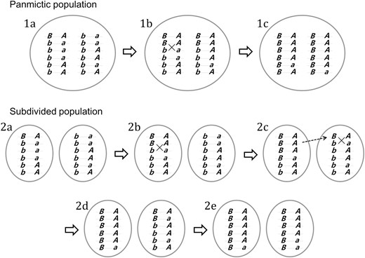
Schematic illustration of the two-locus two-allele model of selective sweeps in panmictic and subdivided (K = 2) populations. Chromosomes found in populations are shown to carry alleles at a locus under selection (wild-type allele b or beneficial allele B) and a neutral locus (allele A or a). The panmictic population is initially fixed for the b allele and a single copy of the B allele appears on a chromosome carrying allele A (the “hitchhiker” allele), which exists in equal frequency with a (stage 1a). The frequency of haplotype BA thus increases rapidly under positive selection and limited recombination. It is shown that a BA chromosome undergoes recombination with a ba chromosome to allow the spread of Ba haplotype in the population (1b indicated by “×”). Allele a thus survives the wipeout but exists in low frequency when B reaches fixation (1c). In the subdivided population, the rapid spread of B, also in association with A, is initially limited to the first deme (2a and 2b). While B is increasing in frequency, its association with A is broken by recombination (2b) and a chromosome carrying the B and the A allele migrates to the second deme and starts increasing there (2c). B in the second deme is also subject to recombination with a (2c). B is fixed in the first deme while it is still in intermediate frequency in the second deme (2d). When B becomes fixed in the entire population (2e), allele a is in low frequency in both demes. Note that it could have been a Ba chromosome instead of a BA chromosome that migrated (in stage 2c) and initiated the spread of B in the second deme, in which case allele a would become dominant in the second deme and result in much less change in the overall allele frequency at the neutral locus in the entire population.

In our model of a subdivided population, 2NK haploid individuals are subdivided equally into K demes. Unless stated otherwise, demes are structured according to the circular stepping-stone model if K > 2. Demes are indexed by 1 to K, indicating their spatial order. Demes 1 and K are neighboring each other, thus making a circular population structure. Generations are not overlapping and, in each generation, haploids reproduce in the order of selection, recombination, and migration. During migration, the proportion m of haploids in deme j moves to neighboring demes (m/2 to deme j − 1 and m/2 to deme j + 1). Note that for K = 2, two demes exchange 2Nm migrants per generation. For modeling the hitchhiking effect, we consider two biallelic loci—selected and neutral loci that are partially linked with the probability of recombination r per generation. At the selected locus, mutation from the wild-type allele b to a beneficial allele B, with selective advantage s, arises on a particular chromosome in deme 1. At the time of this mutation, each of K demes is polymorphic at the neutral locus, with A and a alleles in frequencies p₀ and 1 − p₀, respectively. After genetic hitchhiking, the frequency of A in deme j changes to p_j and p = ∑_jp_j/K. We are mainly concerned about the change in heterozygosity in the entire population (from $\tilde{H} = 2 p_{0} (1 - p_{0})$ to $H^{(T)} = 2 p (1 - p))$ ⁠.

A forward-in-time simulation is built directly on this discrete-time genetic model. At each generation, haplotype frequencies at K demes are changed deterministically by selection, recombination, and migration, followed by the step of random sampling that uses a random binominal number generator (Kim and Wiehe 2009). The initial allele frequency at the neutral locus is given as a fixed value (0.2) for all demes. We also specified initial frequencies for K demes sampled from equilibrium distribution at the balance of mutation, migration, and drift (obtained by separate forward-in-time simulations) but this did not yield different outcomes when the hitchhiking effect was measured by $H^{(T)} / \tilde{H}$ (data not shown). Initial haplotypes were given such that it simulates the occurrence of a beneficial mutation at a randomly chosen chromosome. If the beneficial mutation is lost, the simulation run is repeated from a new initial condition until it reaches fixation in the entire population. All simulation results are based on 10,000 replicates for each parameter combination.

Migration-Limited Trajectory of Beneficial Mutation

The frequency of beneficial mutation rapidly increases within a deme by positive selection. However, its spread into the entire population might be limited by the rate of migration between demes. Namely, there might be a “delay” in the fixation of beneficial mutation in a subdivided population compared to the panmictic population of equal size. To analyze the hitchhiking effect in this model, we first need to understand how much delay in the spread of beneficial mutation is caused by geographical structure of the population. We first consider the case of K = 2. It is assumed that the beneficial mutation arising in deme 1 is eventually fixed in both demes 1 and 2. Let X_j(T) be the frequency of allele B in deme j at time T, when time is counted forward in generations and T = 0 when the mutation to allele B happened in deme 1. Then, we define

{\overset{⌣}{T}}_{j}

= {max}_{T} [X_{j} (T) > 0 and X_{j} (T - 1) = 0]

⁠. Namely,

{\overset{⌣}{T}}_{j}

marks the time when the copy of allele B that survives loss by genetic drift is established in deme j. We define the delay in the spread of allele B by

δ = | {\overset{⌣}{T}}_{2} - {\overset{⌣}{T}}_{1} | .

(1)

(Note that, with m << s,

{\overset{⌣}{T}}_{2} > {\overset{⌣}{T}}_{1} = 0

in most cases. However, with more frequent migration, deme 1 may lose the B allele by genetic drift but later receive the allele from deme 2. In this case the roles of deme 1 and 2 are reversed and the delay becomes

{\overset{⌣}{T}}_{1} - {\overset{⌣}{T}}_{2}

⁠.)

The expected value of δ can be solved by approximating X₁(T) by the deterministic trajectory of a beneficial mutation, starting from frequency ε (<<1), in a single panmictic population of size 2N. It is therefore assumed that migration between two populations does not affect the trajectory, which might be justified for m < s. Therefore, we define

X_{1} (T) = \frac{ε}{ε + \exp (- s T)}

(2)

(Stephan et al. 1992). In each generation, on average 2NmX₁(T) copies of allele B enter deme 2 from deme 1. Each copy of B is lost by genetic drift with probability 1 − 2s, approximately, assuming s << 1. At least one copy of B successfully establishes in deme 2 at time T with probability

1 - {(1 - 2 s)}^{2 N m X_{1} (T)}

⁠. Therefore, the mean waiting time until the first occurrence of such a migrant copy is given by (using

\sum_{n = 1}^{\infty} n (1 - a_{n}) \prod_{i = 0}^{n - 1} a_{i} = \sum_{n = 1}^{\infty} \prod_{i = 0}^{n} a_{i}

if

| a_{n} | < 1

for all n, and making a Taylor series approximation)

\begin{array}{l} E [δ] = {\sum_{T = 1}^{\infty} T (1 - {(1 - 2 s)}^{2 N m X_{1} (T)}) \prod_{i = 0}^{T - 1} (1 - 2 s)}^{2 N m X_{1} (i)} \\ = \sum_{T = 1}^{\infty} {\prod_{i = 0}^{T} (1 - 2 s)}^{2 N m X_{1} (i)} \\ \approx \sum_{T = 1}^{\infty} \exp (- 4 N s m \sum_{i = o}^{T} X_{1} (i)) \\ \approx \int_{0}^{\infty} \exp (- 4 N s m Y_{1} (T)) d T . \end{array}

Here,

\begin{array}{l} Y_{1} (T) = \sum_{i = 0}^{T} X_{1} (i) \\ \approx \int_{0}^{T} X_{1} (z) d z = \int_{0}^{T} \frac{ε}{ε + e^{- s z}} d z = \frac{1}{s} \log (\frac{1 + ε e^{s T}}{1 + ε}) . \end{array}

Therefore,

E [δ] \approx {\int_{0}^{\infty} (\frac{1 + ε}{1 + ε e^{s T}})}^{4 N m} d T \approx \int_{0}^{\infty} \frac{1}{{(1 + ε e^{s T})}^{4 N m}} d T \equiv \bar{δ} .

(3)

An essentially identical result was obtained by Slatkin (1976). With 4Nm ≫1, $\bar{δ}$ is mostly determined by the above integration in the interval [0, $- (1 / s) \ln ε$ ], where we may use (1 + εe^sT)⁴^Nm ≈ 1 + 4Nmεe^sT. Then, a simpler approximation (however, an overestimate of $\bar{δ}$ ⁠) is obtained as

\hat{δ} \equiv \int_{0}^{\infty} \frac{1}{1 + 4 N m ε e^{s T}} d T = \frac{1}{s} \log (\frac{4 N m ε + 1}{4 N m ε}) .

(4)

Considering that the allele frequency of a beneficial mutation starting from one copy is elevated by the inverse of its fixation probability (i.e., probability of surviving extinction by genetic drift ≈ 2s) relative to its deterministic trajectory, we may use ε = 1/(2N)/(2s) = 1/(4Ns) to maximize the fit of Equation 1 to the stochastic trajectory of allele B (Maynard Smith 1971; Kim and Nielsen 2004). Then, we obtain the approximation of the mean delay time

\hat{δ} \equiv \frac{1}{s} \log (1 + \frac{s}{m}) .

(5)

This result shows that the delay time is on the same order (1/s) as the duration of the fixation process (⁠

τ = - (2 / ε) \log (ε))

and critically depends on the relative ratio of s and m. Figure 2 shows the comparison of these approximations to the delay time observed in frequency-based stochastic simulations.

Figure 2

Open in new tab Download slide

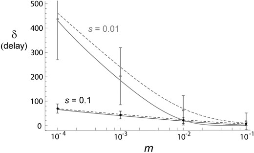
Delay in the spread of a beneficial mutation in a subdivided population with two demes as the function of migration rate, for s = 0.01 (gray) and 0.1 (black) and 2N = 10⁴. Expected delay, $\bar{δ}$ ⁠, by Equation 3 is shown by solid curves and its approximation, $\hat{δ}$ ⁠, is given by dashed curves. Results from frequency-based forward simulations (mean ± SD) are also shown.

Hitchhiking Effect of the Beneficial Mutation—“Marked” Coalescent

Next, we analyze the hitchhiking effect of a beneficial mutation that spreads across demes in the manner described above. Our goal is to obtain an approximate solution for the change of heterozygosity due to hitchhiking. The analysis is based on modeling genetic hitchhiking by the “marked” coalescent, which is derived from the structural coalescent model of genetic hitchhiking (Kaplan et al. 1989). In the structural coalescent model, gene lineages at a neutral locus traced from a present-day sample into the past are described to jump between two genetic backgrounds (corresponding to beneficial, B, and ancestral, b, alleles) by recombination, while coalescence among lineages is allowed only when they are on the same background. It can be shown that, during the selective phase (the period between the birth and fixation of the B allele), lineages that arrive in the b background rarely move back to the B background and also rarely coalesce to each other (Kaplan et al. 1989; Durrett and Schweinsberg 2004; Etheridge et al. 2006; Pfaffelhuber et al. 2006). If we thus model that lineages moving from the B to the b background by recombination remain distinct until they exit the selective phase, the genealogy at the neutral locus is fully described by events of such recombination mapped along the genealogy at the selected locus (referred to below as the B genealogy). Therefore, one may first obtain a B genealogy and then calculate how often it is marked by recombination events to predict the pattern of genetic variation at a linked neutral locus (Pfaffelhuber et al. 2006). Here we first show how a marked coalescent allows a simple derivation of the standard result of genetic hitchhiking [hard selective sweep in a single random mating population (Maynard Smith and Haigh 1974)].

As we are interested in obtaining the heterozygosity after the fixation of the beneficial mutation, we obtain the B genealogy starting from two distinct beneficial mutations on sampled chromosomes. We consider a single panmictic population of size 2N in which the beneficial mutation is quasi-fixed with frequency 1 − ε. Time, t, is now counted backward in generations, t = 0 being the present (time of sampling). Then, the frequency of beneficial mutation, B, in the population is modeled to decrease from 1 − ε to ε by

x (t) = \frac{ε}{ε + \exp (- s (τ - t))}, (0 \leq t \leq τ),

(6)

where

τ = - (2 / ε) \log (ε)

specifies the time when the B allele is introduced in the population. The lineages of the two B alleles will coalesce at t = t_C (≤τ). While tracing each lineage of B, the associated allele at the neutral locus may recombine onto a chromosome carrying allele b at some time between t = 0 and t_C. The probability that this event happens at time t, given that it did not happen in the previous t − 1 generations, is (1 − x(t))r, which is an increasing function with t. If no recombination event occurs on either lineage, the two linked neutral lineages will coalesce at t = t_C, which happens with probability P_coal,

P_{coal} = \int_{0}^{τ} f_{c} (t) {\prod_{z = 0}^{t} (1 - (1 - x (z)) r)}^{2} d t,

(7)

where f_c(t) is the probability distribution of the coalescent time at the selected locus. It is given approximately by

f_{c} (t) = \frac{1}{2 N x (t)} \prod_{i = 0}^{t - 1} (1 - \frac{1}{2 N x (i)}), (0 \leq t \leq τ) .

(8)

This function has a peak close to τ. Then, we may further approximate f_c(t) to be 1 for t = τ and 0 for t < τ − 1: the coalescent occurs at the time of beneficial mutation. This is equivalent to ignoring genetic drift within the allelic class of B (Maynard Smith and Haigh 1974; Barton 1998; Nielsen et al. 2005). Then,

\begin{array}{l} P_{coal} \approx {\prod_{t = 0}^{τ} (1 - (1 - x (t)) r)}^{2} \approx \exp (- 2 r \int_{0}^{τ} (1 - x (t)) d t) \\ = \exp (- 2 r \int_{0}^{τ} \frac{\exp (- s (τ - t))}{ε + \exp (- s (τ - t))} d t) = ε^{2 r / s} . \end{array}

(9)

Ignoring the probability of mutation in the period between t = 0 and τ, the two neutral alleles in the sample will be observed different only if their ancestors at t = τ are distinct, which happens with probability 1 − P_coal, and different. Let $\tilde{H}$ be the expected heterozygosity at the neutral locus at t = τ. Then, the mean heterozygosity at the neutral locus at present is given approximately by

H = \tilde{H} (1 - ε^{2 r / s}) .

(10)

Using ε = 1/(2N), we obtain the solution of Maynard Smith and Haigh (1974). As explained above, a better solution that corrects for the stochastic effect of conditioning on the fixation of beneficial mutation is obtained by using ε = 1/(4Ns), which agrees reasonably well with stochastic simulation results (Kim and Nielsen 2004). More accurate solutions available so far effectively take the full distribution of the coalescent time (Equation 8) (Stephan et al. 1992; Barton 1998) and furthermore the full stochastic trajectory of beneficial mutation (Barton 1998; Etheridge et al. 2006; Pfaffelhuber et al. 2006) into account. However, in this study, we aim to derive solutions for the accuracy of simple approximation $H / \tilde{H} = 1 - {(4 N s)}^{- 2 r / s}$ ⁠, i.e., ignoring genetic drift within the subpopulation of beneficial alleles, as our primary aim is to examine the relative strengths of hitchhiking in panmictic vs. subdivided populations.

Hitchhiking Effect in a Subdivided Population, K = 2

Next, we come back to the model of a subdivided population with K = 2 in which a beneficial mutation, B, arising first in deme 1, propagates into deme 2 with a delay of δ generations. We assume that m < s << 1 but 4Nm >> 1. With this migration rate, the pattern of variation at a neutral locus without selection is close to that of neutral equilibrium in a panmictic population. We thus assume that the heterozygosity at the neutral locus immediately before the time of beneficial mutation (t = δ + τ as defined below) is given by $\tilde{H}$ regardless of whether two chromosomes are sampled from deme 1 only, deme 2 only, or from demes 1 and 2, respectively. However, the corresponding expected heterozygosities may not be equal after the allele B is fixed in the entire population. We denote them as H⁽¹¹⁾, H⁽²²⁾, and H⁽¹²⁾, respectively.

Again, time is counted backward from the present (t = 0), at which the allele B is fixed in the entire population and two haploids are sampled randomly. Assuming migration is weaker than selection (once a copy of B enters a deme, its frequency increases mostly due to selection without being affected by continuous in- and outflow of B), we may model the trajectory of allele B frequency in deme 1 and deme 2 by

x_{1} (t) = \frac{ε}{ε + \exp (- s (τ + δ - t))}, (0 \leq t \leq τ + δ)

(11)

and

x_{2} (t) = (\begin{matrix} \frac{ε}{ε + \exp (- s (τ - t))}, & (0 \leq t \leq τ) \\ 0, & (τ < t \leq τ + δ), \end{matrix}

(12)

respectively. On the basis of this trajectory of the frequency of B, its hitchhiking effect on the neutral locus is determined by first obtaining the coalescent tree at the selected locus and then marking the recombination events on this tree. Below, approximations are obtained for strong selection relative to migration. The lineage of a copy of a B allele (a “B lineage”) in deme 1 will jump to deme 2 with probability ∼2Nmx₂(t + 1)/(2Nx₁(t)) ≈ mx₂(t)/x₁(t) and that in deme 2 will jump to deme 1 with probability ∼mx₁(t)/x₂(t). Then, if selection is strong such that m << 1/τ (but still Nm > 1), migrations of B lineages in either direction will be rare until x₂(t) becomes close to zero, which drastically increases the migration rate from deme 2 to deme 1. On the other hand, if the strength of selection is moderate such that m > 1/τ ≈ s/log[4Ns], there might be multiple jumps of B lineages in both directions between times 0 and τ. To derive simple approximations, we mainly consider the range of large s/m (or m ≪ 1/τ). The applicability of our approximations to a wider parameter range is examined by computer simulations. We also provide an alternative derivation for m > 1/τ in the Appendix.

i. Two gene copies from deme 2

As will be demonstrated shortly, the effect of population subdivision on the hitchhiking effect, examined by relative reduction in expected heterozygosity, may be most pronounced in deme 2 (i.e., effect on $H^{(22)} / \tilde{H}$ ⁠). Consider a sampling of two chromosomes from deme 2 (choosing two of three lineages shown in Figure 3). The “B genealogy” is determined as we trace the lineages of two B alleles on these chromosomes backward in time until they coalesce. Two mutually exclusive genealogical events occur. One event is the separate migrations of two lineages, from deme 2 and deme 1, followed by the coalescence in deme 1. The other event is the coalescence of two lineages in deme 2, followed by the migration of the common ancestor into deme 1. As m ≪ 1/τ, we ignore the possibility that a B lineage migrates to deme 1 and then later migrates back to deme 2 and coalesces. Therefore, once any of these two lineages migrates to deme 1, the coalescence of the two lineages should happen in deme 1. The coalescence in deme 1 must occur before t = τ + δ and that in deme 2 before t = τ . The probabilities of these two events are given by 1 − Q and Q, respectively.

Figure 3

Open in new tab Download slide

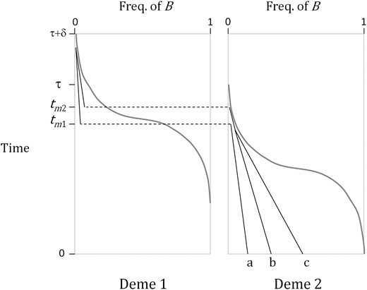
Gene genealogy at the locus under positive directional selection in a subdivided population. Time is counted backward from present (time 0). Gray curves show the frequency trajectory of allele B. Three lineages traced from three chromosomes that are sampled in deme 2 are labeled by a, b, and c. The a and b lineages coalesce in deme 1 after they migrate to deme 1 at time t_m₁ and t_m₂, respectively. The b and c lineages coalesce in deme 2.

Again, the probability that a given lineage in deme 2 migrates to deme 1 is ∼mx₁(t)/x₂(t). The probability that two lineages at deme 2, which remained distinct until time t − 1, coalesce at time t is 1/(2Nx₂(t)). Then, the probability that the coalescent event occurs at deme 2 at time t is given by

\begin{array}{l} f_{2 c} (t) = \frac{1}{2 N x_{2} (t)} \prod_{i = 0}^{t - 1} (1 - \frac{1}{2 N x_{2} (i)} - \frac{2 m x_{2} (i)}{x_{2} (i)}) \\ \approx \frac{1}{2 N x_{2} (t)} \exp [- \sum_{i = 0}^{t - 1} (\frac{1}{2 N x_{2} (i)} + \frac{2 m x_{1} (i)}{x_{2} (i)})] \\ \approx \frac{1}{2 N x_{2} (t)} \exp [- \int_{0}^{t} \frac{1 + 4 N m x_{2} (z)}{2 N x_{2} (z)} d z] \\ = \frac{1}{2 N x_{2} (t)} x_{1} {(t)}^{(2 m / s) (e^{s δ} - 1)} \\ \times \exp [- (2 m + \frac{1}{2 N}) t - \frac{s}{2 N s} (e^{s t} - 1)] . \end{array}

(13)

The total probability of the coalescence in deme 2 is therefore

Q = \sum_{t = 1}^{τ} f_{2 c} (t) \approx \int_{0}^{τ} f_{2 c} (t) d t .

(14)

With probability 1 − Q, the coalescence of B lineages occurs at deme 1. In this case, it is modeled that one B lineage first migrates to deme 1 at time t_m₁ and the other later at t_m₂ (t_m₁ < t_m₂). The probability distribution of t_m₁ is obtained using a similar approximation as

\begin{array}{l} f_{m 1} (t) = P r o b [t_{m 1} = t] \approx \frac{2 m x_{1} (t)}{x_{2} (t)} \prod_{i = 0}^{t - 1} (1 - \frac{1}{2 N x_{2} (i)} - \frac{2 m x_{1} (i)}{x_{2} (i)}) \\ \approx \frac{2 m}{x_{2} (t)} x_{1} (t) 1 + (2 m / s) (e^{s δ} - 1) \\ \times \exp [- (2 m + \frac{1}{2 N}) t - \frac{ε}{2 N s} (e^{s t} - 1)] \\ } = 4 N m x_{1} (t) f_{2 c} (t) . \end{array}

(15)

Figure 4 shows that the peaks of f₂_c(t) and f_m₁(t) both occur between τ/2 and τ. It is because both probabilities for the coalescent and migration increase substantially when x₂(t) becomes small. Given the first migration occurs at t_m₁, t_m₂ should be distributed between t_m₁ and τ. However, as m ≪ 1/τ we may assume that t_m₂ is simply equal to τ (the remaining B lineage traces back to the first B allele that, forward in time, entered deme 2 and survived stochastic loss). As demonstrated below, this simplification leads to an overestimation of heterozygosity at the linked neutral locus. Furthermore, we make another simplifying assumption that two B lineages now in deme 1 coalesce at time t = τ + δ, which also leads to an overestimation of heterozygosity at the neutral locus by the same degree that Equation 10 overestimates the heterozygosity in the standard (panmixia) model of genetic hitchhiking.

Figure 4

Probability of coalescence and lineage migration as functions of time. The gray curve, the black curve, and the gray dashed curve plot f2c(t) (Equation 13), fm1(t) (Equation 15), and fm(t) (Equation 20), respectively. The x-axis shows scaled time (backward) during the selective phase, with 0 and 1 corresponding to unscaled time 0 and τ (= 1520), respectively, with K = 2, 2N = 105, s = 0.01, and m = 10−4. The peaks of fm1(t) and fm(t) move closer to 1.0 (τ) as m is further reduced (not shown).

Open in new tab Download slide

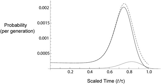
Probability of coalescence and lineage migration as functions of time. The gray curve, the black curve, and the gray dashed curve plot f₂_c(t) (Equation 13), f_m₁(t) (Equation 15), and f_m(t) (Equation 20), respectively. The x-axis shows scaled time (backward) during the selective phase, with 0 and 1 corresponding to unscaled time 0 and τ (= 1520), respectively, with K = 2, 2N = 10⁵, s = 0.01, and m = 10⁻⁴. The peaks of f_m₁(t) and f_m(t) move closer to 1.0 (τ) as m is further reduced (not shown).

Heterozygosity at the neutral locus is determined by the probability that the B genealogy described above is marked by a recombination event by which a linked neutral lineage moves to a chromosome carrying allele b. The probability of this recombination event at time t is (1 − x₁(t))r if the lineage is in deme 1 and (1 − x₂(t))r if the lineage is in deme 2. Therefore, no recombination event is marked on a lineage that remains in deme i from time t₁ to t₂ with probability $\prod_{t = t_{1}}^{t_{2}} {1 - r (1 - x_{i} (t))} \approx \exp [- r \int_{t_{1}}^{t_{2}} (1 - x_{i} (t)) d t] .$ Given that B lineages coalesce at deme 1 (with probability $\int_{0}^{r} f_{m 1} (t) d t = 1 - Q$ ⁠), the probability that this genealogy is marked by zero recombination events (i.e., neutral lineages coalesce at the same time B lineages coalesce) is approximated by

\begin{matrix} P_{coal}^{(1)} = \int_{0}^{τ} f_{m 1} (t) \exp [- r \int_{0}^{t} (1 - x_{2} (z)) d z - r \int_{t}^{τ + δ} (1 - x_{1} (z)) d z \\ - r \int_{0}^{τ} (1 - x_{2} (z)) d z - r \int_{τ}^{τ + δ} (1 - x_{1} (z)) d z] d t / (1 - Q) \\ = \int_{0}^{τ} f_{m 1} (t) {(\frac{1 + ε e^{s t}}{1 + ε}) (\frac{1 + ε e^{s τ}}{1 + ε e^{s (t - δ)}}) (\frac{1 + ε e^{s τ}}{1 + ε}) (\frac{1 + ε e^{s τ}}{1 + ε e^{s (τ - δ)}})}^{- (r / s)} d t / (1 - Q) \\ = {(\frac{1 + ε}{ε^{2} (ε + e^{- s δ})})}^{- (r / s)} \int_{0}^{τ} f_{m 1} (t) {(\frac{x_{1} (t)}{x_{2} (t)})}^{- (r / s)} d t / (1 - Q) . \end{matrix}

(16)

If δ is smaller than τ/2 (i.e., $ε ≪ e^{- s δ}$ ⁠), we get

P_{coal}^{(1)} \approx ε^{2 r / s} e^{- r δ} \int_{0}^{τ} f_{m 1} (t) {(\frac{x_{1} (t)}{x_{2} (t)})}^{- (r / s)} d t / (1 - Q) .

(17)

If t_m₁ ≈ τ (for very small m), $P_{coal}^{(1)}$ is further approximated to $ε^{2 r / s} e^{- 2 r δ},$ as $x_{1} (τ) \approx ε e^{s δ} .$ Therefore, the hitchhiking effect (the relative reduction in heterozygosity at the neutral locus) given such genealogy at the selected locus is ∼ $1 - ε^{2 r / s} e^{- 2 r δ} .$ Compared with the solution in the panmixia model of hitchhiking (Equation 10), the homozygosity decreases by a factor of $e^{- 2 r δ},$ which clearly represents the additional opportunity for recombination due to the extended length of B genealogy (= δ) due to migration. {Note that more accurate comparison between panmictic vs. subdivided populations should take the difference in ε [e.g., 1/(8Ns) vs. 1/(4Ns), respectively, for a total population size of 4N] into account. Therefore, the comparison in this case should be made between 1 − (ε/2)²^r^/^s and $1 - ε^{2 r / s} e^{- 2 r δ} .$ }

If δ >> τ [ $ε ≫ e^{- s δ}$ and x₁(r) ≈ 1], Equation 16 is similarly approximated to ε⁴^r^/^s, which basically means a twofold increase in the neutral lineages’ opportunity to dissociate from B lineages. However, this radical effect on genetic hitchhiking may not happen frequently because δ ≫ τ requires a very low migration rate, which causes B lineages to coalesce in deme 2 rather than in deme 1.

If B lineages coalesce in deme 2, the probability that this genealogy is marked by zero recombination events is approximated by

\begin{array}{l} P_{coal}^{(2)} = \frac{\int_{0}^{τ} f_{c} (t) \exp [- 2 r \int_{0}^{t} (1 - x_{2} (z)) d z] d t}{Q} \\ = \frac{\int_{0}^{τ} f_{c} (t) {((1 + ε e^{s t}) / (1 + ε))}^{- (2 r / s)} d t}{Q}, \end{array}

(18)

which is slightly greater than ε²^r^/^s as the time of the coalescent is smaller than τ. Finally, the hitchhiking effect on the heterozygosity for two gene copies sampled in deme 2 is given by

\frac{H^{(22)}}{\tilde{H}} = (1 - Q) (1 - P_{coal}^{(1)}) + Q (1 - P_{coal}^{(2)}) .

(19)

Figures 5 and 6 show the comparison between this approximation and results from frequency-based simulation. As we took steps in simplifying formulas that consistently lead to the overestimation of relative heterozygosity after a selective sweep, our approximation predicts greater elevation of heterozygosity (i.e., greater decline of the hitchhiking effect) due to population subdivision than suggested by simulation results.

Figure 5

Relative heterozygosity (H(22) /H˜) for two chromosomes sampled in deme 2 with increasing recombination from the selected locus. Analytic approximations and the results of frequency-based simulations are shown for an identical set of parameters [2N = 105, s = 0.01 (black) or 0.1 (gray), and m/s = 0.01]. On the left, solid and dashed curves show the hitchhiking effect in the subdivided (K = 2) population [Equation 19 using δ=δ¯ (Equation 3)] and in the panmictic population (1−(8Ns)−r/s), respectively. Corresponding simulation results are shown on the right.

Open in new tab Download slide

Relative heterozygosity $(H^{(22)} / \tilde{H})$ for two chromosomes sampled in deme 2 with increasing recombination from the selected locus. Analytic approximations and the results of frequency-based simulations are shown for an identical set of parameters [2N = 10⁵, s = 0.01 (black) or 0.1 (gray), and m/s = 0.01]. On the left, solid and dashed curves show the hitchhiking effect in the subdivided (K = 2) population [Equation 19 using $δ = \bar{δ}$ (Equation 3)] and in the panmictic population $(1 - {(8 N s)}^{- r / s}),$ respectively. Corresponding simulation results are shown on the right.

Figure 6

The relative effect of population subdivision [H(22)subdiv/H(22)panmic] for two chromosomes sampled from deme 2 as a function of migration rate. K = 2, 2N = 105, r/s = 0.01, and s = 0.01 (black) and 0.1 (gray). Approximations are given by the ratio of Equation 19 with δ=δ¯ and 1−(8Ns)−r/s. Heterozygosity (mean ± 2 SE) obtained in the simulation of the subdivided population (K = 2) was divided by the mean heterozygosity obtained from the simulation of genetic hitchhiking in the panmictic population (the population with 4N chromosomes).

Open in new tab Download slide

The relative effect of population subdivision [H⁽²²⁾_subdiv/H⁽²²⁾_panmic] for two chromosomes sampled from deme 2 as a function of migration rate. K = 2, 2N = 10⁵, r/s = 0.01, and s = 0.01 (black) and 0.1 (gray). Approximations are given by the ratio of Equation 19 with $δ = \bar{δ}$ and $1 - {(8 N s)}^{- r / s} .$ Heterozygosity (mean ± 2 SE) obtained in the simulation of the subdivided population (K = 2) was divided by the mean heterozygosity obtained from the simulation of genetic hitchhiking in the panmictic population (the population with 4N chromosomes).

ii. One gene copy from deme 1 and the other from deme 2

Next, the approximate solution for the expected heterozygosity when one chromosome is sampled from deme 1 and the other from deme 2, H⁽¹²⁾, is similarly obtained. Ignoring the possibility that the B lineage starting in deme 1 enters deme 2 and coalesces to the other B lineage there, we may consider a model in which the coalescence of two B lineages occurs in deme 1 only: one lineage always remains in deme 1 and the other lineage migrates from deme 2 to deme 1 at time t_m. This will lead to an overestimation of H⁽¹²⁾ because the coalescence in deme 2, which would produce smaller B genealogy with less opportunity for recombination, is precluded. Furthermore, we again make the simplifying assumption that the coalescent event in deme 1 happens at t = τ + δ. Then, the probability that this genealogy is marked by zero recombination events is approximately

\begin{array}{l} P_{coal}^{(12)} = \int_{0}^{τ} f_{m} (t) \exp [- r \int_{0}^{τ + δ} (1 - x_{1} (z)) d z \\ - r \int_{0}^{t} (1 - x_{2} (z)) d z - r \int_{t}^{τ + δ} (1 - x_{1} (z)) d z] d t \\ = \int_{0}^{τ} f_{m} (t) {(\frac{ε + 1}{ε + e^{- s (τ + δ)}}) (\frac{ε + e^{- s (τ - t)}}{ε + e^{- s τ}}) (\frac{ε + 1}{ε + e^{- s (τ + δ - t)}})}^{- (r / s)} d t \\ \approx ε^{2 r / s} {\int_{0}^{τ} f_{m} (t) (\frac{x_{1} (t)}{x_{2} (t)})}^{- (r / s)} d t, \end{array}

(20)

where f_m(t) is the probability distribution of t_m. Therefore,

H^{(12)} \approx \tilde{H} (1 - ε^{2 r / s} \int_{0}^{τ} f_{m} (t) {(\frac{x_{1} (t)}{x_{2} (t)})}^{- (r / s)} d t) .

(21)

We may use

\begin{array}{l} f_{m} (t) \approx \frac{2 m x_{1} (t)}{x_{2} (t)} \prod_{i = 0}^{t - 1} (1 - \frac{2 m x_{1} (i)}{x_{2} (i)}) \\ \approx \frac{2 m x_{1} (t)}{x_{2} (t)} \exp [- 2 m \int_{0}^{t} \frac{x_{1} (z)}{x_{2} (z)} d z] \\ = \frac{2 m}{x_{2} (t)} x_{1} {(t)}^{1 + (2 m / s) (e^{s δ} - 1)} e^{- 2 m t} . \end{array}

(22)

However, when m/s is very small, which causes the distribution of t_m to be sharply concentrated very closely to τ, the above equation fails to accurately describe the probability density (data not shown). We thus take another step of simplification by using f_m(t) = 1 if t = τ and 0 otherwise: the migration of the lineage from deme 2 to 1 happens at time τ. This again leads to the overestimation of H⁽¹²⁾ because the length of the lineage staying in deme 2 and being subject to recombination marking is maximized. H⁽¹²⁾ is then finally reduced to

H^{(12)} \approx \tilde{H} (1 - ε^{2 r / s} e^{- r δ}),

(23)

assuming

x_{1} (τ) \approx ε e^{s δ} .

The factor

e^{- r δ}

indicates that only one B lineage, starting from deme 2, is subject to the additional marking of a recombination event due to its extension by δ. Figure 7 shows the analytic approximation to the relative increase of H⁽¹²⁾ due to population subdivision [Equation 23, with

δ = \bar{δ},

divided by

\tilde{H} (1 - {(ε / 2)}^{2 r / s}),

which is the prediction for panmixia after merging demes 1 and 2] and the corresponding quantity observed in simulations. As expected, our approximation overestimates the elevation of H⁽¹²⁾ caused by population subdivision.

Figure 7

The relative effect of population subdivision [H(12)subdiv/H(12)panmic] for a pair of chromosomes sampled from different demes as a function of migration rate. K = 2, 2N = 105, r/s = 0.01, and s = 0.01 (black) and 0.1 (gray). Approximations are given by the ratio of Equation 23 with δ=δ¯ and 1−(8Ns)−r/s. Heterozygosity (mean ± 2 SE) obtained in the simulation of the subdivided population (K = 2) was divided by the mean heterozygosity obtained from the simulation of genetic hitchhiking in the panmictic population (the population with 4N chromosomes).

Open in new tab Download slide

The relative effect of population subdivision [H⁽¹²⁾_subdiv/H⁽¹²⁾_panmic] for a pair of chromosomes sampled from different demes as a function of migration rate. K = 2, 2N = 10⁵, r/s = 0.01, and s = 0.01 (black) and 0.1 (gray). Approximations are given by the ratio of Equation 23 with $δ = \bar{δ}$ and $1 - {(8 N s)}^{- r / s} .$ Heterozygosity (mean ± 2 SE) obtained in the simulation of the subdivided population (K = 2) was divided by the mean heterozygosity obtained from the simulation of genetic hitchhiking in the panmictic population (the population with 4N chromosomes).

iii. Two gene copies from deme 1

We finally investigate the expected heterozygosity when both chromosomes are sampled from deme 1. When it is assumed that lineages starting in deme 1 do not migrate to deme 2, the hitchhiking effect is determined solely due to the trajectory of B in deme 1 only. In that case

H^{(11)} \approx \tilde{H} (1 - ε^{2 r / s}),

(24)

which is basically the result of a selective sweep as it occurs in deme 1 in isolation. Note that this level of heterozygosity is lower than that in the panmictic population that would be created if two demes are merged via free migration. The latter is given by

\tilde{H} (1 - {(ε / 2)}^{2 r / s})

because the initial frequency of B is halved as the population size doubles. It is well known that, if all else is equal, reduction in polymorphism by a single selective sweep is greater in a smaller population because the frequency trajectory of the beneficial allele is shorter (Barton 2000). Therefore, the effect of population subdivision with low migration is to increase the hitchhiking effect when two chromosomes are sampled from the deme where the beneficial allele originated. However, as the migration rate increases, H⁽¹¹⁾ should approach that in the merged panmictic population. Therefore, it is expected that the relative effect of population subdivision on hitchhiking, H⁽¹¹⁾_subdiv/H⁽¹¹⁾_panmic, is ∼(1−ε²^r^/^s)/(1−(ε/2)²^r^/^s) with m ≪ 1/τ but gradually increases to 1 as m increases. Simulation results confirm this prediction (Figure 8). In the following, we use Equation 24 for H⁽¹¹⁾ as we are mainly concerned in the case of m≪s.

Figure 8

The relative effect of population subdivision [H(11)subdiv/H(11)panmic] for two chromosomes sampled from deme 1 as a function of migration rate. K = 2, 2N = 105, r/s = 0.01, and s = 0.01 (black) and 0.1 (gray). Dashed-dotted lines mark the approximate low-migration limit of the heterozygosity ratio: (1 − ε2r/s)/(1 − (ε/2)2r/s) (see text for explanation). Heterozygosity (mean ± 2 SE) obtained in the simulation of the subdivided population (K = 2) was divided by the mean heterozygosity obtained from the simulation of genetic hitchhiking in the panmictic population (the population with 4N chromosomes).

Open in new tab Download slide

The relative effect of population subdivision [H⁽¹¹⁾_subdiv/H⁽¹¹⁾_panmic] for two chromosomes sampled from deme 1 as a function of migration rate. K = 2, 2N = 10⁵, r/s = 0.01, and s = 0.01 (black) and 0.1 (gray). Dashed-dotted lines mark the approximate low-migration limit of the heterozygosity ratio: (1 − ε²^r^/s)/(1 − (ε/2)²^r^/s) (see text for explanation). Heterozygosity (mean ± 2 SE) obtained in the simulation of the subdivided population (K = 2) was divided by the mean heterozygosity obtained from the simulation of genetic hitchhiking in the panmictic population (the population with 4N chromosomes).

iv. Random sample from the entire population

The expected effect of hitchhiking on the entire population, given that two chromosomes are sampled randomly over two demes, is therefore

\frac{H^{(T)}}{\tilde{H}} = (\frac{H^{(11)}}{4} + \frac{H^{(12)}}{2} + \frac{H^{(22)}}{4}) / \tilde{H} .

(25)

Figures 9 and 10 show that the relative heterozygosity after genetic hitchhiking is larger in the subdivided population with small m than in the panmictic population. Namely, population subdivision weakens the strength of genetic hitchhiking. Compared to simulation results, our approximation overestimates the elevation of relative heterozygosity for small m, as expected from our consistent use of assumptions that lead to the overestimation of heterozygosity. However, we also note that this effect of population subdivision is limited to very small m/s values. With intermediate m (∼0.1s), both the approximation (although expected to be inaccurate) and simulation results suggest that only minor elevation of heterozygosity occurs. An alternative derivation for m > 1/τ, provided in the Appendix, also suggests that no significant increase of heterozygosity occurs due to population subdivision.

Figure 9

Relative heterozygosity (H(T) /H˜) for two chromosomes randomly sampled from the entire population with increasing recombination from the selected locus. Analytic approximations and the results of frequency-based simulations are shown for an identical set of parameters [2N = 105, s = 0.01 (black) or 0.1 (gray), and m/s = 0.01]. On the left, solid and dashed curves show the hitchhiking effect in the subdivided (K = 2) population [Equation 25 in which H(11), H(12), and H(22) are given by Equations 24, 23, and 19, respectively, and δ=δ¯] and that in the panmictic population (1−(8Ns)−r/s), respectively. Corresponding simulation results are shown on the right.

Open in new tab Download slide

Relative heterozygosity $(H^{(T)} / \tilde{H})$ for two chromosomes randomly sampled from the entire population with increasing recombination from the selected locus. Analytic approximations and the results of frequency-based simulations are shown for an identical set of parameters [2N = 10⁵, s = 0.01 (black) or 0.1 (gray), and m/s = 0.01]. On the left, solid and dashed curves show the hitchhiking effect in the subdivided (K = 2) population [Equation 25 in which H⁽¹¹⁾, H⁽¹²⁾, and H⁽²²⁾ are given by Equations 24, 23, and 19, respectively, and $δ = \bar{δ}$ ] and that in the panmictic population $(1 - {(8 N s)}^{- r / s}),$ respectively. Corresponding simulation results are shown on the right.

Figure 10

Open in new tab Download slide

The relative effect of population subdivision [H⁽^T⁾_subdiv/H⁽^T⁾_panmic and the relative increase of fixation time] for a pair of chromosomes randomly sampled from the entire population as a function of migration rate. K = 2, 2N = 10⁵, r/s = 0.01, and s = 0.01 (black) and 0.1 (gray). Approximations for heterozygosity ratio (solid curves) are obtained by Equation 25 divided by $1 - {(8 N s)}^{- r / s},$ where $δ = \bar{δ}$ and H⁽¹¹⁾, H⁽¹²⁾, and H⁽²²⁾ are given by Equations 24, 23, and 19, respectively. Heterozygosity (mean ± 2 SE) obtained in the simulation of the subdivided population (K = 2) was divided by the mean heterozygosity obtained from the simulation of genetic hitchhiking in the panmictic population (the population with 4N chromosomes). Dashed curves show $(\bar{δ} + 2 \log [4 N s] / 2) / (2 \log [8 N s] / s),$ the expectation for the relative increase in time taken for the beneficial allele to become fixed in the entire population.

We also plotted in Figure 10 the expected increase in time taken for a beneficial mutation to become fixed in the entire population (“fixation time”), given by the ratio of the expectation under population subdivision, $\bar{δ} + 2 \log [4 N s] / 2,$ and that under panmixia, 2 log[8Ns]/s. As the relative length of the fixation time increases in the subdivided population with decreasing m, $H^{(T)} / \tilde{H}$ also increases. This result is compatible with the conjecture that the extension of fixation time allows more recombination that breaks the association between beneficial and neutral alleles. However, decreasing the migration rate has a greater effect on fixation time than on heterozygosity. Figures 6 and 7 show that H⁽²²⁾ and H⁽¹²⁾ respond differently to decreasing m, the overall effect being less drastic increase of H⁽^T⁾ than that of fixation time.

Subdivided Population With K = 10

Next, we expand our analysis to the stepping-stone model of a subdivided population with more than two demes. The beneficial mutation arising in deme 1 is expected to propagate symmetrically in both directions and the last deme where the mutation is fixed is ⌊K/2⌋ steps away from deme 1. We therefore predict that, at least for m ≪ s, the mean total time taken for the beneficial mutation to become fixed in the entire population (fixation time” is approximately

τ_{K} = \bar{δ} ⌊ \frac{K}{2} ⌋ + \frac{2 \log [4 N s]}{s} .

(26)

Compared to simulation results, this approximation works well asymptotically for very small m/s while the panmictic approximation works for larger m (Figure 11). As the migration rate increases, the fixation time approaches that in the corresponding panmictic population.

Figure 11

Open in new tab Download slide

Time taken for a beneficial mutation to become fixed in the subdivided population with K = 10, as the function of migration rate. Simple approximation (Equation 26; black curve) is compared with simulation results (gray curve). 2N = 10⁵ and s = 0.01. Mean values were obtained from 10,000 replicates for each parameter set. The expected time for the corresponding panmictic population, 2 log[4NKs]/s, is shown by the dashed line.

Simulation results were obtained only for the hitchhiking effect with K = 10. The pattern of heterozygosity immediately after the fixation of the beneficial allele in the entire population is similar to that with K = 2 (Figure 12A): a smaller migration rate between neighboring demes results in higher heterozygosity (for two chromosomes randomly selected from the entire population; shaded curve in Figure 12A). However, similar to the case of K = 2, the elevation of heterozogosity is less pronounced than the increase of fixation time. For example, comparing Figures 11 and 12A, while fixation time increases by 68%, heterozygosity increases by 34%. When two chromosomes are sampled from each subpopulation, heterozygosity greatly depends on the location of sampling if m ≪ s: heterozygosity is lowest in the deme of the beneficial mutation’s origin (deme 1) and progressively increases as distance from deme 1 increases (Figure 12A). This generalizes the pattern obtained above with K = 2 that the strength of genetic hitchhiking diminishes as the beneficial mutation spreads across neighboring demes. As explained above, genetic hitchhiking reduces heterozygosity in the first deme of a subdivided population with small m/s more than it reduces heterozygosity in the merged (panmictic) population because deme 1 behaves similarly to a small isolated population. However, in other demes (e.g., demes 3–6 in Figure 12A), heterozygosity greatly increases as migration rate decreases. This produces an overall negative correlation between heterozygosity (over the entire population) and migration rate. We also note that, as migration rate decreases, heterozygosity over the entire population increases much faster than heterozygosity for a single deme. This reflects the fact that genetic hitchhiking spreading over a subdivided population creates genetic differentiation among subpopulations that were initially homogeneous (see below), as predicted by Slatkin and Wiehe (1998).

Figure 12

Relative heterozygosity (H(.) /H˜) for two chromosomes randomly sampled within individual demes (from deme 1 to deme 6 shown by curves with increasing dash sizes) and from the entire population (gray curve) for the stepping-stone model (A) and the island model (B) with K = 10 and r/s = 0.01. Note that, for the stepping-stone model, the fixation of the beneficial mutation occurs first in deme 1 and last in deme 6. Parameters for simulations are identical to those used for simulations described in Figure 11.

Open in new tab Download slide

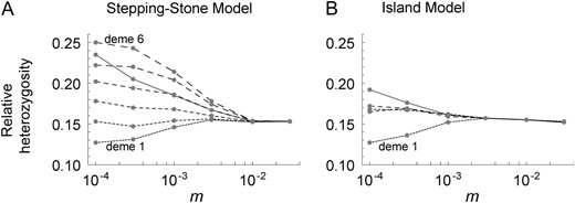
Relative heterozygosity $(H^{(.)} / \tilde{H})$ for two chromosomes randomly sampled within individual demes (from deme 1 to deme 6 shown by curves with increasing dash sizes) and from the entire population (gray curve) for the stepping-stone model (A) and the island model (B) with K = 10 and r/s = 0.01. Note that, for the stepping-stone model, the fixation of the beneficial mutation occurs first in deme 1 and last in deme 6. Parameters for simulations are identical to those used for simulations described in Figure 11.

For a comparison, we also simulated selective sweeps spreading over K = 10 demes that are arranged according to Wright’s island model, in which a given haploid chromosome enters a common migrant pool with probability m per generation and then migrates to a randomly chosen deme. Except for this change in spatial arrangement, the same sets of parameters used in the simulations of the stepping-stone model were used. Figure 12B shows that the mean heterozygosity over the entire population after a selective sweep (shaded curve) increases with decreasing m. However, this increase is much smaller than that for the stepping-stone model. Similar to the stepping-stone model, the mean heterozygosity in deme 1, the birthplace of the beneficial allele, is reduced with low migration. Mean heterozygosities in other demes (results for only three of nine demes are shown in Figure 12B) slightly increase with decreasing migration. Much smaller heterozygosity for an individual deme than that for the entire population again reflects genetic differentiation among demes. Comparing Figure 12A and 12B, we conclude that the pattern of a selective sweep is more severely affected in the stepping-stone model than in the island model, which demonstrates the complexity of genetic hitchhiking caused by a beneficial mutation that spreads in one-dimensional space.

Further results, regarding the variance of heterozygosity and population differentiation, from the simulation of the stepping-stone model are given in Table 1. The coefficient of variation, $c v_{i j} = \sqrt{Var [H^{(i j)}]} / \bar{H^{(i j)}},$ where H⁽^ij⁾ is the expected heterozygosity for one chromosome sampled in deme i and another in deme j, was obtained over 10,000 replicates for a given parameter set. We also calculated F_ST = (H⁽^T⁾ − H⁽^S⁾)/H⁽^T⁾, where H⁽^T⁾ is the expected heterozygosity in the entire population and $H^{(S)} = (\sum_{i = 1}^{K} H^{(i i)}) / K .$ It is shown that, for a given r/s, population subdivision (reduction in m) causes a moderate increase in the coefficient of variation while it causes a drastic increase in F_ST. Note that simulation started with uniform frequencies of a neutral allele in all demes (F_ST = 0). As predicted by Slatkin and Wiehe (1998) and Bierne (2010), the effect of population subdivision on genetic differentiation after a selective sweep critically depends on the recombination rate: Table 1 shows that, for a given m, intermediate values of r/s (0.03 ∼ 0.1) produce the largest F_ST.

Simulation of stepping-stone model (K = 10, s = 0.01, 2N = 10⁵)

Table 1

Simulation of stepping-stone model (K = 10, s = 0.01, 2N = 10⁵)

r/s	m/s	H⁽¹¹⁾ (cv₁₁)	H⁽³³⁾ (cv₃₃)	H⁽⁶⁶⁾ (cv₆₆)	H⁽¹³⁾ (cv₁₃)	H⁽¹⁶⁾ (cv₁₆)	H⁽³⁶⁾ (cv₃₆)	F_ST
0.01	0.01	0.041 (1.81)	0.057 (1.72)	0.080 (1.51)	0.057 (1.78)	0.082 (1.76)	0.089 (1.65)	0.068
0.01	0.03	0.042 (1.66)	0.054 (1.60)	0.078 (1.43)	0.052 (1.59)	0.070 (1.55)	0.075 (1.49)	0.037
0.01	0.1	0.047 (1.49)	0.054 (1.45)	0.069 (1.33)	0.052 (1.43)	0.061 (1.36)	0.064 (1.35)	0.015
0.01	0.3	0.045 (1.40)	0.051 (1.39)	0.057 (1.33)	0.051 (1.38)	0.054 (1.33)	0.055 (1.34)	0.0047
0.01	1	0.049 (1.34)	0.049 (1.34)	0.049 (1.34)	0.049 (1.34)	0.049 (1.34)	0.049 (1.33)	0.00086
0.001	0.1	0.0049 (4.18)	0.0054 (4.27)	0.0077 (4.06)	0.0053 (4.03)	0.0066 (3.99)	0.0069 (4.03)	0.0060
0.003	0.1	0.014 (2.52)	0.016 (2.51)	0.022 (2.36)	0.016 (2.44)	0.019 (2.42)	0.020 (2.37)	0.0088
0.01	0.1	0.047 (1.49)	0.054 (1.45)	0.069 (1.33)	0.052 (1.43)	0.061 (1.36)	0.064 (1.35)	0.015
0.03	0.1	0.119 (0.95)	0.133 (0.92)	0.161 (0.84)	0.130 (0.92)	0.149 (0.87)	0.155 (0.86)	0.022
0.1	0.1	0.246 (0.55)	0.258 (0.52)	0.281 (0.43)	0.257 (0.52)	0.276 (0.48)	0.279 (0.46)	0.021
0.3	0.1	0.312 (0.23)	0.313 (0.21)	0.316 (0.17)	0.315 (0.20)	0.319 (0.16)	0.319 (0.16)	0.0098
1	0.1	0.317 (0.14)	0.317 (0.14)	0.318 (0.14)	0.319 (0.11)	0.321 (0.10)	0.320 (0.10)	0.0063

r/s	m/s	H⁽¹¹⁾ (cv₁₁)	H⁽³³⁾ (cv₃₃)	H⁽⁶⁶⁾ (cv₆₆)	H⁽¹³⁾ (cv₁₃)	H⁽¹⁶⁾ (cv₁₆)	H⁽³⁶⁾ (cv₃₆)	F_ST
0.01	0.01	0.041 (1.81)	0.057 (1.72)	0.080 (1.51)	0.057 (1.78)	0.082 (1.76)	0.089 (1.65)	0.068
0.01	0.03	0.042 (1.66)	0.054 (1.60)	0.078 (1.43)	0.052 (1.59)	0.070 (1.55)	0.075 (1.49)	0.037
0.01	0.1	0.047 (1.49)	0.054 (1.45)	0.069 (1.33)	0.052 (1.43)	0.061 (1.36)	0.064 (1.35)	0.015
0.01	0.3	0.045 (1.40)	0.051 (1.39)	0.057 (1.33)	0.051 (1.38)	0.054 (1.33)	0.055 (1.34)	0.0047
0.01	1	0.049 (1.34)	0.049 (1.34)	0.049 (1.34)	0.049 (1.34)	0.049 (1.34)	0.049 (1.33)	0.00086
0.001	0.1	0.0049 (4.18)	0.0054 (4.27)	0.0077 (4.06)	0.0053 (4.03)	0.0066 (3.99)	0.0069 (4.03)	0.0060
0.003	0.1	0.014 (2.52)	0.016 (2.51)	0.022 (2.36)	0.016 (2.44)	0.019 (2.42)	0.020 (2.37)	0.0088
0.01	0.1	0.047 (1.49)	0.054 (1.45)	0.069 (1.33)	0.052 (1.43)	0.061 (1.36)	0.064 (1.35)	0.015
0.03	0.1	0.119 (0.95)	0.133 (0.92)	0.161 (0.84)	0.130 (0.92)	0.149 (0.87)	0.155 (0.86)	0.022
0.1	0.1	0.246 (0.55)	0.258 (0.52)	0.281 (0.43)	0.257 (0.52)	0.276 (0.48)	0.279 (0.46)	0.021
0.3	0.1	0.312 (0.23)	0.313 (0.21)	0.316 (0.17)	0.315 (0.20)	0.319 (0.16)	0.319 (0.16)	0.0098
1	0.1	0.317 (0.14)	0.317 (0.14)	0.318 (0.14)	0.319 (0.11)	0.321 (0.10)	0.320 (0.10)	0.0063

Open in new tab

Table 1

Simulation of stepping-stone model (K = 10, s = 0.01, 2N = 10⁵)

r/s	m/s	H⁽¹¹⁾ (cv₁₁)	H⁽³³⁾ (cv₃₃)	H⁽⁶⁶⁾ (cv₆₆)	H⁽¹³⁾ (cv₁₃)	H⁽¹⁶⁾ (cv₁₆)	H⁽³⁶⁾ (cv₃₆)	F_ST
0.01	0.01	0.041 (1.81)	0.057 (1.72)	0.080 (1.51)	0.057 (1.78)	0.082 (1.76)	0.089 (1.65)	0.068
0.01	0.03	0.042 (1.66)	0.054 (1.60)	0.078 (1.43)	0.052 (1.59)	0.070 (1.55)	0.075 (1.49)	0.037
0.01	0.1	0.047 (1.49)	0.054 (1.45)	0.069 (1.33)	0.052 (1.43)	0.061 (1.36)	0.064 (1.35)	0.015
0.01	0.3	0.045 (1.40)	0.051 (1.39)	0.057 (1.33)	0.051 (1.38)	0.054 (1.33)	0.055 (1.34)	0.0047
0.01	1	0.049 (1.34)	0.049 (1.34)	0.049 (1.34)	0.049 (1.34)	0.049 (1.34)	0.049 (1.33)	0.00086
0.001	0.1	0.0049 (4.18)	0.0054 (4.27)	0.0077 (4.06)	0.0053 (4.03)	0.0066 (3.99)	0.0069 (4.03)	0.0060
0.003	0.1	0.014 (2.52)	0.016 (2.51)	0.022 (2.36)	0.016 (2.44)	0.019 (2.42)	0.020 (2.37)	0.0088
0.01	0.1	0.047 (1.49)	0.054 (1.45)	0.069 (1.33)	0.052 (1.43)	0.061 (1.36)	0.064 (1.35)	0.015
0.03	0.1	0.119 (0.95)	0.133 (0.92)	0.161 (0.84)	0.130 (0.92)	0.149 (0.87)	0.155 (0.86)	0.022
0.1	0.1	0.246 (0.55)	0.258 (0.52)	0.281 (0.43)	0.257 (0.52)	0.276 (0.48)	0.279 (0.46)	0.021
0.3	0.1	0.312 (0.23)	0.313 (0.21)	0.316 (0.17)	0.315 (0.20)	0.319 (0.16)	0.319 (0.16)	0.0098
1	0.1	0.317 (0.14)	0.317 (0.14)	0.318 (0.14)	0.319 (0.11)	0.321 (0.10)	0.320 (0.10)	0.0063

r/s	m/s	H⁽¹¹⁾ (cv₁₁)	H⁽³³⁾ (cv₃₃)	H⁽⁶⁶⁾ (cv₆₆)	H⁽¹³⁾ (cv₁₃)	H⁽¹⁶⁾ (cv₁₆)	H⁽³⁶⁾ (cv₃₆)	F_ST
0.01	0.01	0.041 (1.81)	0.057 (1.72)	0.080 (1.51)	0.057 (1.78)	0.082 (1.76)	0.089 (1.65)	0.068
0.01	0.03	0.042 (1.66)	0.054 (1.60)	0.078 (1.43)	0.052 (1.59)	0.070 (1.55)	0.075 (1.49)	0.037
0.01	0.1	0.047 (1.49)	0.054 (1.45)	0.069 (1.33)	0.052 (1.43)	0.061 (1.36)	0.064 (1.35)	0.015
0.01	0.3	0.045 (1.40)	0.051 (1.39)	0.057 (1.33)	0.051 (1.38)	0.054 (1.33)	0.055 (1.34)	0.0047
0.01	1	0.049 (1.34)	0.049 (1.34)	0.049 (1.34)	0.049 (1.34)	0.049 (1.34)	0.049 (1.33)	0.00086
0.001	0.1	0.0049 (4.18)	0.0054 (4.27)	0.0077 (4.06)	0.0053 (4.03)	0.0066 (3.99)	0.0069 (4.03)	0.0060
0.003	0.1	0.014 (2.52)	0.016 (2.51)	0.022 (2.36)	0.016 (2.44)	0.019 (2.42)	0.020 (2.37)	0.0088
0.01	0.1	0.047 (1.49)	0.054 (1.45)	0.069 (1.33)	0.052 (1.43)	0.061 (1.36)	0.064 (1.35)	0.015
0.03	0.1	0.119 (0.95)	0.133 (0.92)	0.161 (0.84)	0.130 (0.92)	0.149 (0.87)	0.155 (0.86)	0.022
0.1	0.1	0.246 (0.55)	0.258 (0.52)	0.281 (0.43)	0.257 (0.52)	0.276 (0.48)	0.279 (0.46)	0.021
0.3	0.1	0.312 (0.23)	0.313 (0.21)	0.316 (0.17)	0.315 (0.20)	0.319 (0.16)	0.319 (0.16)	0.0098
1	0.1	0.317 (0.14)	0.317 (0.14)	0.318 (0.14)	0.319 (0.11)	0.321 (0.10)	0.320 (0.10)	0.0063

Open in new tab

Discussion

Complex geographic and demographic structures of natural populations have potentially great impact on evolutionary genetic processes and thus on the interpretation of DNA sequence polymorphism (Jensen et al. 2005; Nielsen et al. 2005; Li and Stephan 2006; Kim and Gulisija 2010; Stephan 2010). To examine the effect of spatial demographic structure on the pattern of selective sweeps, we used a simplified model of population subdivision. While a relatively slow evolutionary process such as the coalescence of neutral gene lineages may be less sensitive to spatial structure, a fast nonequilibrium process that sweeps across the entire population can be greatly affected by population subdivision, as demonstrated in this study. On the basis of results obtained above, we find that population subdivision causes several important modifications in the strength and pattern of a selective sweep.

First, the strength of genetic hitchhiking, measured by the reduction of expected heterozygosity, is diminished in a subdivided population if the migration rate is much smaller than the selective advantage of the beneficial mutation, while the population structure shaped by the same migration rate might be undetected in the examination of neutral polymorphism. As briefly argued by Barton (2000), this effect is attributed to increased time taken for the beneficial mutation to reach high frequency, which provides more opportunity for the breakdown of hitchhiking by recombination. This result implies that the strength of directional selection estimated from the chromosomal span of reduced polymorphism (Kim and Stephan 2002; Thornton et al. 2007) assuming panmixia might be an underestimate. However, we also find that the relative increase in the fixation time of a beneficial mutation under population subdivision is much greater than the relative increase in expected heterozygosity. This implies that, if the strength of selection is estimated separately from the chromosomal span of reduced polymorphism and from the age of the sweeping haplotype estimated by rare mutations (for example, Sáez et al. 2003; Meiklejohn et al. 2004; Xue et al. 2006), the former estimate might be greater than the latter (and closer to the true value). It is not, however, clear whether such a discrepancy can be detected with a reasonable statistical power.

The second important result is that a beneficial mutation leaves weaker signature of selection as it spreads across distant demes after its origin in the first population. With K = 2, while population subdivision results in a much stronger hitchhiking effect in the first population relative to that expected under panmixia (Equation 24 with m ≪ s), it causes a much weaker hitchhiking effect in the second population: the relative level of expected polymorphism is much higher than the panmixia. It is because the extension of neutral lineages exposed to hitchhike-breaking recombination applies only to those descending to the second population. Comparing Figures 6 and 8 we find that the expected heterozygosity can be up to 30% higher in the second population than in the first. Figure 12A also indicates that a gradient of heterozygosity will be observed along the path of the beneficial mutation’s propagation in a geographically structured population. Slatkin and Wiehe (1998) and Bierne (2010) showed that genetic hitchhiking can introduce population differentiation (large F_ST) in an initially homogeneous population (small F_ST) and also implicitly suggested that this population differentiation occurs as a selective sweep leaves asymmetric levels of variation in accordance with our conclusion. Their and our results make it clear that an evolutionary process can lead to heterogeneous outcomes across different demes if it occurs faster than migration. We may use this prediction of the gradient of heterozygosity along the pathway of a sweep to infer the geographical origin of a beneficial mutation and reveal the pattern of migration in a hidden geographic structure by analyzing DNA sequence polymorphism that harbors a signature of selective sweep distributed over multiple demes.

This study used simple models of a structured population, in which demes are of equal size and a given structure of division remains unchanged through time. Actual populations in nature experience complex demographic changes. An important case of demographic complexity is the split of an ancestral population into several demes that are dispersed over geographic structure, as in the evolutionary history of humans. We argue that our analysis of selective sweeps in subdivided populations is still applicable to this demographic scenario. If a beneficial mutation spreads very rapidly across subpopulations, which should be true for strong selection even with a certain delay by limited migration, the selective sweep would effectively occur under constant geographic structure as the timescale of the sweep is much shorter than that of major demographic processes. Our analysis can be applied as long as demes are genetically homogeneous at the time of mutation to the beneficial allele. This condition will be met if different demes were recently established from the split of the ancestral population and thus contain similar profiles of genetic variation.

Although it was not explicitly addressed in this study, our analysis suggests that population subdivision may also significantly modify the other (“higher-order”) pattern of polymorphism as the signature of a selective sweep. The site frequency spectrum and linkage disequilibrium are critically dependent on the shape (branching pattern) of the coalescent trees at the neutral loci, which in turn depends on the shape of genealogy at the locus under selection (B genealogy) (Fay and Wu 2000; Kim and Nielsen 2004; McVean 2007; Pfaffelhuber et al. 2008). For example, Pfaffelhuber et al. (2006) showed that approximating the B genealogy by a Yule process corrects the error introduced by the assumption of star-like B genealogy. Population subdivision is likely to introduce a much greater deviation from the star-like genealogy that cannot be corrected by a Yule tree. Consider a sample of chromosomes that are distributed randomly over multiple demes. The probability that two B lineages coalesce in a deme outside its mutational origin (Equation 14), thus preventing a star-like tree, becomes nonnegligible if s is sufficiently larger than m. Furthermore, while the markings of recombination events are concentrated near the root of a Yule tree in a single panmictic population, it is expected to occur in many other points along a B genealogy, corresponding to times when a B lineage is in a deme with low frequency of B, in a subdivided population. How these factors modify the patterns of frequency spectrum and linkage disequilibrium, particularly along the demes in the path of beneficial mutation’s propagation, remains to be investigated. This requires the development of computer simulation methods that can generate multisite (realistic DNA sequence) polymorphism data, which is planned for a follow-up article.

Acknowledgements

We thank Wolfgang Stephan and two anonymous reviewers whose comments greatly improved the manuscript. This work was supported by National Institutes Health grant R01GM084320 and an Ewha Womans University Research Grant of 2010.

Footnotes

Communicating editor: M. W. Feldman

Literature Cited

Akey

J M

,

2009

Constructing genomic maps of positive selection in humans: Where do we go from here?

Genome Res.

19

:

711

–

722

.

Baines

J F

,

Das

A

,

Mousset

S

,

Stephan

W

,

2004

The role of natural selection in genetic differentiation of worldwide populations of Drosophila ananassae

.

Genetics

168

:

1987

–

1998

.

Barton

N H

,

1998

The effect of hitch-hiking on neutral genealogies

.

Genet. Res.

72

:

123

–

133

.

Google Scholar

Crossref

WorldCat

Barton

N H

,

2000

Genetic hitchhiking

.

Philos. Trans. R. Soc. B Biol. Sci.

355

:

1553

.

Google Scholar

Crossref

WorldCat

Bierne

N

,

2010

The distinctive footprints of local hitchhiking in a varied environment and global hitchhiking in a subdivided population

.

Evolution

64

:

3254

–

3272

.

Das

A

,

Mohanty

S

,

Stephan

W

,

2004

Inferring population structure and demography of Drosophila ananassae from multilocus data

.

Genetics

168

:

1975

–

1985

.

Durrett

R

,

Schweinsberg

J

,

2004

Approximating selective sweeps

.

Theor. Popul. Biol.

66

:

129

–

138

.

Etheridge

A

,

Pfaffelhuber

P

,

Wakolbinger

A

,

2006

An approximate sampling formula under genetic hitchhiking

.

Ann. Appl. Probab.

16

:

685

–

729

.

Google Scholar

Crossref

WorldCat

Faure

M F

,

David

P

,

Bonhomme

F

,

Bierne

N

,

2008

Genetic hitchhiking in a subdivided population of Mytilus edulis

.

BMC Evol. Biol.

8

:

164

.

Fay

J C

,

Wu

C I

,

2000

Hitchhiking under positive Darwinian selection

.

Genetics

155

:

1405

–

1413

.

Hermisson

J

,

Pennings

P S

,

2005

Soft sweeps: molecular population genetics of adaptation from standing genetic variation

.

Genetics

169

:

2335

–

2352

.

Jensen

J D

,

Kim

Y

,

Dumont

V B

,

Aquadro

C F

,

Bustamante

C D

,

2005

Distinguishing between selective sweeps and demography using DNA polymorphism data

.

Genetics

170

:

1401

–

1410

.

Kaplan

N L

,

Hudson

R R

,

Langley

C H

,

1989

The “hitchhiking effect” revisited

.

Genetics

123

:

887

–

899

.

Kim

Y

,

Gulisija

D

,

2010

Signatures of recent directional selection under different models of population expansion during colonization of new selective environments

.

Genetics

184

:

571

–

585

.

Kim

Y

,

Nielsen

R

,

2004

Linkage disequilibrium as a signature of selective sweeps

.

Genetics

167

:

1513

–

1524

.

Kim

Y

,

Stephan

W

,

2002

Detecting a local signature of genetic hitchhiking along a recombining chromosome

.

Genetics

160

:

765

–

777

.

Kim

Y

,

Wiehe

T

,

2009

Simulation of DNA sequence evolution under models of recent directional selection

.

Brief. Bioinform.

10

:

84

–

96

.

Li

H

,

Stephan

W

,

2006

Inferring the demographic history and rate of adaptive substitution in Drosophila

.

PLoS Genet.

2

:

e166

.

Maynard Smith

J

,

1971

What use is sex

.

J. Theor. Biol.

30

:

319

–

335

.

Maynard Smith

J

,

Haigh

J

,

1974

The hitch-hiking effect of a favorable gene

.

Genet. Res.

23

:

23

–

35

.

McVean

G

,

2007

The structure of linkage disequilibrium around a selective sweep

.

Genetics

175

:

1395

.

Meiklejohn

C D

,

Kim

Y

,

Hartl

D L

,

Parsch

J

,

2004

Identification of a locus under complex positive selection in Drosophila simulans by haplotype mapping and composite-likelihood estimation

.

Genetics

168

:

265

–

279

.

Nielsen

R

,

2005

Molecular signatures of natural selection

.

Annu. Rev. Genet.

39

:

197

–

218

.

Nielsen

R

,

Williamson

S

,

Kim

Y

,

Hubisz

M J

,

Clark

A G

et al. ,

2005

Genomic scans for selective sweeps using SNP data

.

Genome Res.

15

:

1566

.

Pfaffelhuber

P

,

Haubold

B

,

Wakolbinger

A

,

2006

Approximate genealogies under genetic hitchhiking

.

Genetics

174

:

1995

–

2008

.

Pfaffelhuber

P

,

Lehnert

A

,

Stephan

W

,

2008

Linkage disequilibrium under genetic hitchhiking in finite populations

.

Genetics

179

:

527

.

Sabeti

P C

,

Schaffner

S F

,

Fry

B

,

Lohmueller

J

,

Varilly

P

et al. ,

2006

Positive natural selection in the human lineage

.

Science

312

:

1614

–

1620

.

Sáez

A G

,

Tatarenkov

A

,

Barrio

E

,

Becerra

N H

,

Ayala

F J

,

2003

Patterns of DNA sequence polymorphism at Sod vicinities in Drosophila melanogaster: unraveling the footprint of a recent selective sweep

.

Proc. Natl. Acad. Sci. USA

100

:

1793

–

1798

.

Google Scholar

Crossref

WorldCat

Santiago

E

,

Caballero

A

,

2005

Variation after a selective sweep in a subdivided population

.

Genetics

169

:

475

–

483

.

Slatkin

M

,

1976

The rate of spread of an advantageous allele in a subdivided population

, pp.

767

–

780

in

Population Genetics and Ecology

, edited by

Karlin

S

,

Nevo

E

.

Academic Press

,

New York

.

Slatkin

M

,

1987

Gene flow and the geographic structure of natural populations

.

Science

236

:

787

.

Slatkin

M

,

Wiehe

T

,

1998

Genetic hitch-hiking in a subdivided population

.

Genet. Res.

71

:

155

–

160

.

Stephan

W

,

2010

Detecting strong positive selection in the genome

.

Mol. Ecol. Res.

10

:

863

–

872

.

Google Scholar

Crossref

WorldCat

Stephan

W

,

Wiehe

T H E

,

Lenz

M W

,

1992

The effect of strongly selected substitutions on neutral polymorphism: analytical results based on diffusion-theory

.

Theor. Popul. Biol.

41

:

237

–

254

.

Google Scholar

Crossref

WorldCat

Stephan

W

,

Xing

L

,

Kirby

D A

,

Braverman

J M

,

1998

A test of the background selection hypothesis based on nucleotide data from Drosophila ananassae

.

Proc. Natl. Acad. Sci. USA

95

:

5649

–

5654

.

Google Scholar

Crossref

WorldCat

Thornton

K R

,

Jensen

J D

,

Becquet

C

,

Andolfatto

P

,

2007

Progress and prospects in mapping recent selection in the genome

.

Heredity

98

:

340

–

348

.

Williamson

S H

,

Hubisz

M J

,

Clark

A G

,

Payseur

B A

,

Bustamante

C D

et al. ,

2007

Localizing recent adaptive evolution in the human genome

.

PLoS Genet.

3

:

e90

.

Wright

S

,

1940

Breeding structure of populations in relation to speciation

.

Am. Nat.

74

:

232

–

248

.

Google Scholar

Crossref

WorldCat

Xue

Y

,

Daly

A

,

Yngvadottir

B

,

Liu

M

,

Coop

G

et al. ,

2006

Spread of an inactive form of caspase-12 in humans is due to recent positive selection

.

Am. J. Hum. Genet.

78

:

659

–

670

.

Appendix: Deriving an Approximate Solution to Relative Heterozygosity for τ > 1/m

When s is not large enough to satisfy τ ≪ 1/m, while it may be still greater than m such that δ is nonnegligible, we cannot make the assumption that a B lineage stays in one deme until x₂(t) becomes small. B lineages will jump frequently across demes if m is greater than 1/τ. (For example, with 2N = 10⁵, s = 0.01, and m = 0.001, it is calculated that $\hat{δ} = 182.5$ while τ = 1520 > 1/m.) In such a case, we may ignore the probability that two B lineages will coalesce at deme 2 [Equations 13 and 14 show that Q is a decreasing function of m for a given τ, as the dominant factor of f_c(t) between time 0 and τ/2 is $e^{- 2 m t}$ ]. B lineages are then modeled to coalesce in deme 1 only, approximately at t = τ + δ. Let λ(t) (= 1 or 2) be the location (deme) of a randomly chosen B lineage at time t and I₁[λ] be 1 if λ = 1 and 0 otherwise. Then, considering two randomly chosen chromosomes from the entire population and a very small recombination rate, the probability of the coalescence at the neutral locus is given by

\begin{matrix} P_{coal} = 〈 \prod_{t = 1}^{τ + δ} {1 - I_{1} [λ (t)] r (1 - x_{1} (t)) - (1 - I_{1} [λ (t)]) r (1 - x_{2} (t))}^{2} 〉 \\ \approx 〈 1 - 2 r \sum_{t = 1}^{τ + δ} {I_{1} [λ (t)] (1 - x_{1} (t)) + (1 - I_{1} [λ (t)) (1 - x_{2} (t))} 〉 \\ = 1 - 2 r \sum_{t = 1}^{τ + δ} {〈 I_{1} [λ (t)] 〉 (1 - x_{1} (t)) + (1 - 〈 I_{1} [λ (t)] 〉) (1 - x_{2} (t))}, \end{matrix}

(A1)

where $〈 〉$ indicates the mean obtained by integration over all possible sample paths of λ(t). If the jumps of B lineages are frequent enough, a given lineage would be in deme 1 or deme 2 with probabilities x₁(t)/(x₁(t) + x₂(t)) and x₂(t)/(x₁(t) + x₂(t)), respectively, at time t. Therefore, using an approximation $〈 I_{1} [λ (t)] 〉$ ≈ x₁(t)/(x₁(t) + x₂(t)),

\begin{matrix} P_{coal} \approx 1 - 2 r \sum_{t = 1}^{τ + δ} (1 - x_{1} (t) - x_{2} (t) + \frac{2 x_{1} (t) x_{2} (t)}{x_{1} (t) + x_{2} (t)}) \\ \approx 1 - 2 r \int_{0}^{τ + δ} (1 - x_{1} (t) - x_{2} (t) + \frac{2 x_{1} (t) x_{2} (t)}{x_{1} (t) + x_{2} (t)}) d t \\ = 1 - 2 r (τ + δ) + \frac{2 r}{s} {\log [\frac{1 + ε e^{- s δ}}{ε^{2} e^{- s δ} + ε e^{- s δ}}] + \log [\frac{1 + ε}{ε^{2} e^{- s δ} + ε}] - \log [\frac{2 + ε (1 + e^{- s δ})}{2 ε^{2} e^{- s δ} + ε (1 + e^{- s δ})}]} \\ \approx 1 - 2 r (τ + δ) + \frac{2 r}{s} \log [\frac{e^{s δ} + 1}{2 ε}] \\ \approx \exp [- 2 r (τ + δ) + \frac{2 r}{s} \log [\frac{e^{s δ} + 1}{2 ε}]] \\ = ε^{2 r / s} {(\frac{1 + e^{- s δ}}{2})}^{2 r / s} \approx {(\frac{ε}{2})}^{2 r / s} . \end{matrix}

(A2)

The last approximation results from the earlier assumption that δ is nonnegligible compared to τ $(e^{- s δ} ≪ 1) .$ Therefore, the hitchhiking effect approaches that of the panmictic population that would form if two demes merge. When $e^{- s δ}$ cannot be ignored relative to 1, the above derivation yields P_coal > (ε/2)²^r^/^s, which means a stronger hitchhiking effect under a subdivided population contrary to the expectation that population subdivision would cause an overall increase in heterozygosity (and thus a decrease in homozygosity). Similar to the underestimation of H⁽¹¹⁾ (Equation 24) relative to a panmictic expectation with intermediate m, this error results from specifying the initial frequency of the beneficial mutation in deme 1 to be ε = 1/(4Ns): with frequent migration that satisfies τ > 1/m, the stochastic dynamics of the beneficial mutation would conform to that in a panmictic population of 4N chromosomes. In that case, specifying the initial frequency to be ε would underestimate the length of selective phase, which leads to the overestimation of the hitchhiking effect. In conclusion, this derivation, despite errors, suggests that a clear decline in hitchhiking effect due to population subdivision is not expected under m > 1/τ.

This article is published and distributed under the terms of the Oxford University Press, Standard Journals Publication Model (https://academic.oup.com/journals/pages/open_access/funder_policies/chorus/standard_publication_model)

Download all slides

Month:	Total Views:
January 2021	2
February 2021	1
March 2021	10
April 2021	13
May 2021	9
June 2021	9
July 2021	14
August 2021	3
September 2021	7
October 2021	8
November 2021	10
December 2021	13
January 2022	5
February 2022	27
March 2022	13
April 2022	21
May 2022	17
June 2022	22
July 2022	19
August 2022	25
September 2022	9
October 2022	15
November 2022	18
December 2022	11
January 2023	5
February 2023	6
March 2023	24
April 2023	19
May 2023	10
June 2023	14
July 2023	16
August 2023	6
September 2023	11
October 2023	19
November 2023	27
December 2023	24
January 2024	31
February 2024	20
March 2024	18
April 2024	21

Article Contents

Hitchhiking Effect of a Beneficial Mutation Spreading in a Subdivided Population

Abstract

Model

Migration-Limited Trajectory of Beneficial Mutation

Hitchhiking Effect of the Beneficial Mutation—“Marked” Coalescent

Hitchhiking Effect in a Subdivided Population, K = 2

i. Two gene copies from deme 2

ii. One gene copy from deme 1 and the other from deme 2

iii. Two gene copies from deme 1

iv. Random sample from the entire population

Subdivided Population With K = 10

Simulation of stepping-stone model (K = 10, s = 0.01, 2N = 10⁵)

Discussion

Acknowledgements

Footnotes

Literature Cited

Appendix: Deriving an Approximate Solution to Relative Heterozygosity for τ > 1/m

Citations

Views

Altmetric

Email alerts

Citing articles via

Latest

Most Read

Most Cited

Article Contents

Hitchhiking Effect of a Beneficial Mutation Spreading in a Subdivided Population

Abstract

Model

Migration-Limited Trajectory of Beneficial Mutation

Hitchhiking Effect of the Beneficial Mutation—“Marked” Coalescent

Hitchhiking Effect in a Subdivided Population, K = 2

i. Two gene copies from deme 2

ii. One gene copy from deme 1 and the other from deme 2

iii. Two gene copies from deme 1

iv. Random sample from the entire population

Subdivided Population With K = 10

Simulation of stepping-stone model (K = 10, s = 0.01, 2N = 105)

Discussion

Acknowledgements

Footnotes

Literature Cited

Appendix: Deriving an Approximate Solution to Relative Heterozygosity for τ > 1/m

Citations

Views

Altmetric

Email alerts

Citing articles via

Latest

Most Read

Most Cited

This Feature Is Available To Subscribers Only

Simulation of stepping-stone model (K = 10, s = 0.01, 2N = 10⁵)