Intratumor Heterogeneity in Evolutionary Models of Tumor Progression

Durrett, Rick; Foo, Jasmine; Leder, Kevin; Mayberry, John; Michor, Franziska

doi:10.1534/genetics.110.125724

Abstract

With rare exceptions, human tumors arise from single cells that have accumulated the necessary number and types of heritable alterations. Each such cell leads to dysregulated growth and eventually the formation of a tumor. Despite their monoclonal origin, at the time of diagnosis most tumors show a striking amount of intratumor heterogeneity in all measurable phenotypes; such heterogeneity has implications for diagnosis, treatment efficacy, and the identification of drug targets. An understanding of the extent and evolution of intratumor heterogeneity is therefore of direct clinical importance. In this article, we investigate the evolutionary dynamics of heterogeneity arising during exponential expansion of a tumor cell population, in which heritable alterations confer random fitness changes to cells. We obtain analytical estimates for the extent of heterogeneity and quantify the effects of system parameters on this tumor trait. Our work contributes to a mathematical understanding of intratumor heterogeneity and is also applicable to organisms like bacteria, agricultural pests, and other microbes.

HUMAN cancers frequently display substantial intratumor heterogeneity in genotype, gene expression, cellular morphology, metabolic activity, motility, and behaviors such as proliferation rate, antigen expression, drug response, and metastatic potential (Fidler and Hart 1982; Heppner 1984; Nicolson 1984; Campbell and Polyak 2007; Dick 2008). For example, a molecular and phenotypic analysis of breast cancer cells has revealed defined subpopulations with distinct gene expression and (epi)genetic profiles (Shipitsin et al. 2007). Heterogeneity and the existence of subpopulations within single tumors have also been demonstrated via flow cytometry in cervical cancers and lymph node metastases (Nguyen et al. 1993) as well as in leukemias (Wolman 1986). Virtually every major type of human cancer has been shown to contain distinct cell subpopulations with differing heritable alterations (Heppner 1984; Merlo et al. 2006; Campbell and Polyak 2007). Heterogeneity is also present in premalignant lesions; for instance, genetic clonal diversity has been observed in Barrett's esophagus, a condition associated with increased risk of developing esophageal adenocarcinoma (Maley et al. 2006; Lai et al. 2007).

Tumor heterogeneity has direct clinical implications for disease classification and prognosis as well as for treatment efficacy and the identification of drug targets (Merlo et al. 2006; Campbell and Polyak 2007). The degree of clonal diversity in Barrett's esophagus, for instance, is correlated with clinical progression to esophageal adenocarcinoma (Maley et al. 2006). In prostate carcinomas, tumor heterogeneity plays a key role in pretreatment underestimation of tumor aggressiveness and incorrect assessment of DNA ploidy status of tumors (Wolman 1986; Haggarth et al. 2005). Heterogeneity has long been implicated in the development of resistance to cancer therapies after an initial response (Geisler 2002; Merlo et al. 2006) as well as in the development of metastases (Fidler 1978). In addition, tumor heterogeneity hampers the precision of microarray-based analyses of gene expression patterns, which are widely used for the identification of genes associated with specific tumor types (O'Sullivan et al. 2005). These issues underscore the importance of obtaining a more detailed understanding of the origin and temporal evolution of intratumor heterogeneity.

To study the dynamics of intratumor heterogeneity, we construct and analyze a stochastic evolutionary model of an expanding population with random mutational fitness advances. Evolutionary models of populations with random mutational advances have been studied in the context of fixed-size Wright–Fisher processes for both finite and infinite populations (Gerrish and Lenski 1998; Park and Krug 2007; Park et al. 2010); Gerrish and Lenski (1998) studied the speed of evolution in a Wright–Fisher model with random mutational advances in the context of finite but large populations while Park et al. (2010) obtained accurate asymptotic approximations for the evolutionary dynamics of the population, following ideas presented in Park and Krug (2007). The latter work and references therein constitute a substantial exploration of the effects of random mutational advances in fixed-size populations. Our present work complements this research by exploring the effects of random mutational advances in the context of exponentially expanding populations and in particular the implications of these mutational advances on population heterogeneity. Models of exponentially expanding populations are appropriate for the study of situations arising during tumorigenesis, but are also applicable to other organisms undergoing binary replication such as bacteria, agricultural pests, and other microbes and pathogens. Bacterial populations, for instance, are diverging quickly in both genotype and phenotype, as studied by Lenski and colleagues. These investigators examined the dynamics of phenotypic evolution in populations of Escherichia coli that were propagated by daily serial transfer for 1500 days, yielding 10,000 generations of binary fission (Lenski et al. 1991; Lenski and Travisano 1994). The fitness of the bacteria improved on average by 50% relative to the ancestor, and other phenotypic properties, such as cell size, also underwent large changes. Similarly, single malaria isolates have been found to consist of heterogeneous populations of parasites that can have varying characteristics of drug response, from highly resistant to completely sensitive (Foley and Tilley 1997). These findings have implications for treatment strategies, as not all pathogen populations are sensitive to therapeutic interventions, and necessitate the study of diversity dynamics in growing populations of cells.

In this article, we consider an exponentially expanding population of tumor cells in which (epi)genetic alterations confer random fitness changes to cells. This model is used to investigate the extent of genetic diversity in tumor subpopulations as well as its evolution over time. The mathematical framework is based on the clonal evolution model of carcinogenesis, which postulates that tumors are monoclonal (i.e., originating from a single abnormal cell) and that over time the descendants of this ancestral cell acquire various combinations of mutations (Merlo et al. 2006; Campbell and Polyak 2007). According to this model, genetic drift and natural selection drive the progression and diversity of tumors. Our work complements studies of the effects of random mutational fitness distributions on the growth kinetics of tumors (Durrett et al. 2010) and contributes to the mathematical investigation of intratumor heterogeneity (Coldman and Goldie 1985, 1986; Michelson et al. 1989; Kansal et al. 2000; Komarova 2006; Haeno et al. 2007; Schweinsberg 2008; Bozic et al. 2010; Durrett and Moseley 2010).

MATERIALS AND METHODS

We consider a multitype branching process model of tumorigenesis in which (epi)genetic alterations confer an additive change to the birth rate of the cell. This additive change is drawn according to a probability distribution v, which is referred to as the mutational fitness distribution. Cells that have accumulated i ≥ 0 mutations are denoted as type-i cells. Initially, the population consists entirely of type-0 cells, which divide at rate a₀, die at rate b₀, and produce type-1 cells at rate u. The initial population, whose size is given by V₀, is considered to be sufficiently large so that its growth can be approximated by $Z_{0} (t) = V_{0} \exp [λ_{0} t]$ ⁠, where λ₀ = a₀ − b₀ and time t is measured in units of cell division. Type-1 cells divide at rate a₀ + X, where X ≥ 0 is drawn according to the distribution v, and give rise to type-2 cells at rate u. All cell types die at rate b₀ < a₀. In general, a type-(k − 1) cell with birth rate a_k−₁ produces a new type-k cell at rate u, and the new type-k cell type divides at rate a_k₋₁ +X, where $X \geq 0$ is drawn according to v. Each type-k cell produced by a type-(k − 1) cell initiates a genetically distinct lineage of cells, and the set of all of its type-k descendants is referred to as its family. The total number of type-k cells in the population at time t is given by $Z_{k} (t)$ and the set of all type-k cells is called the kth wave or generation k. The total population size at time t is given by $Z (t)$ ⁠.

Note that in our model, mutations are not coupled to cell divisions but instead occur at a fixed rate per unit of time. This model can be modified to exclusively consider (epi)genetic alterations that occur during cell division by assuming that type-0 individuals divide at rate α₀ and during each division, there is a chance μ that a mutation occurs, producing a type-1 individual. These two model versions are equivalent for wave-1 cells if a₀ = α₀(1 − μ) and u = α₀μ. For later waves, the model must be altered so that the mutation rate is dependent upon the genetic constitution of the cells, since accumulation of alterations modifies the fitness of the cell and hence the rate at which further changes are accumulated. Analysis of this model would then require the mutation rate term to be inside the integral over the support of the fitness distribution; however, this modification does not alter the limiting results significantly. Our model and results can also be modified to account for generation-dependent mutation rates (Coldman and Goldie 1985; Park et al. 2010).

The mutational fitness distribution v determines the effects of each (epi)genetic change that is accumulated in the population of cells. We consider fitness distributions concentrated on [0, b] for some b > 0. We discuss two distinct classes of distributions: (i) v is discrete and assigns mass g_i to a finite number of values $b_{1} < b_{2} < . . . < b_{N} = b$ ⁠; (ii) v is continuous with a bounded density $g (x)$ that is continuous and positive at b. Figure 1 shows a snapshot of the population decomposition in a sample simulation for case ii and illustrates the complex genotypic composition of the population of cells generated by our model.

Figure 1.—

Open in new tab Download slide

A sample cross-section of tumor heterogeneity. (A) The composition of a tumor cell population at $t = 150$ time units after tumor initiation. Each “wave” of cells, defined as the set of cells harboring the same number of (epi)genetic alterations, is represented by a different color. Individual clones of cells with identical genotype are shown as circles, positioned on the horizontal axis according to fitness (i.e., birth rate) and on the vertical axis according to clone size. Note that later waves tend to have larger fitness values. (B) The time at which individual clones of cells were created during tumor progression. The color scale depicts the time of emergence of each clone. In A and B, parameters are $a_{0} = 0.2$ ⁠, $b_{0} = 0.1$ ⁠, $v \sim U ([0, 0.05])$ ⁠, and $u = 0.001.$

The determination of the distribution v in the context of bacteria and viruses has been the subject of several experimental studies (Imhof and Schlotterer 2001; Sanjuan et al. 2004), which have generally produced results leading to the conclusion that v has an exponential distribution. However, more recently Rokyta and colleagues (Rokyta et al. 2008) presented studies of bacteriophages, in which the distribution of beneficial mutational effects appears to have a truncated right tail. One possible explanation for this result is that the experiments were done at an elevated temperature that might have led to a limited number of available beneficial mutations. A similar scenario might arise during tumorigenesis when only a limited number of (epi)genetic alterations allow a cell to progress to a more aggressive phenotype.

RESULTS

There are two sources of heterogeneity present in the population: variability in the number of mutations per cell (heterogeneity between generations) and genotypic variation between members of the same generation (heterogeneity within a generation). We investigate these two sources of heterogeneity and derive analytic results that quantify the relationship between model parameters—e.g., mutation rate and mutational fitness distribution—and the amount of genotypic variation present in the population over time.

Between-generation heterogeneity:

Asymptotic results for the size of generation k were obtained in (Durrett et al. 2010; Durrett and Moseley 2010); see Equations A1 and A2 in the appendix for restatements of the relevant results from these articles. Equation A1 implies that in case i, for example, we have the approximation

\log Z_{k} (t) \approx λ_{k} t - (k + p_{k}) \log (1 / u) + \log V_{d, k},

(2)

when t is large, where

λ_{k} = λ_{0} + k b

is the maximum growth rate that can be attained by generation k mutants,

p_{k} = - k + \frac{\sum_{j = 0}^{k - 1} λ_{k}}{λ_{j}},

and

V_{d, k}

is a positive random variable with known Laplace transform. In case ii there is an additional term in (2) of the form

(k + p_{k}) \log t

⁠. Dividing both sides of (2) by

L = \log (1 / u)

and speeding up time by a factor of L, we note that the log size of generation k approaches a deterministic, linear limit as the mutation rate becomes very small. In particular, as

u \to 0

⁠, we have

(1 / L) \log^{+} Z_{k} (L t) \to z_{k} (t) = {[λ_{k} t - (k + p_{k})]}^{+} = λ_{k} {(t - β_{k})}^{+}

(3a)

in probability, where

β_{k} = \frac{k + p k}{λ_{k}} = \sum_{j = 0}^{k - 1} \frac{1}{λ_{j}} .

(3b)

The limiting process depends on λ₀, the growth rate of type-0 cells, and b, the maximum attainable fitness increase, but is otherwise independent of the particular choice of fitness distribution. An example of the limiting process is displayed in Figure 2, a and b.

Figure 2.—

Open in new tab Download slide

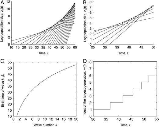
The process for the small mutation limit. The limiting process is shown for the case in which the mutation rate goes to zero. (A) The time, t, on the horizontal axis vs. the log number of cells of wave k, $z_{k} (t)$ ⁠, as given by Equation 3. Both time and space are given in units of L = log(1/u). This plot shows the first 20 waves started at $t = 10 = 1 / λ_{0},$ i.e., the time that type-1 cells begin to be born. (B) A closer look at the first 7 waves from a, showing the changes in the dominant type. (C) The birth times of the first 20 generations as a function of the generation number. (D) The dominant type in the population as a function of time. The index $m (t)$ of the largest generation at time t is defined as $z_{m (t)} (t) = \max {z_{k} (t) : k \geq 0}$ ⁠. In A–D, parameters are $λ_{0} = 0.1$ and $b = 0.05$ ⁠.

As a consequence of Equation 3, we obtain the following insight regarding the birth time of type-k cells: if

T_{k} = \inf {t \geq 0 : Z_{k} (t) > 0}

is the first time a type-k individual is born, then, as

u \to 0

⁠,

\frac{T_{k}}{L} \to β_{k}

(4)

in probability for all k ≥ 0. From the definition of

β_{k}

⁠, we have that

β_{k} - β_{k - 1} = 1 / λ_{k}

is decreasing so that the increments between the birth times for successive generations decrease as k increases. This effect leads to an acceleration in the rate at which new mutations are accumulated (Figure 2c). This acceleration occurs regardless of the choice of fitness distribution, assuming that i or ii holds. Since

1 / λ_{k}

is inversely proportional to b, distributions that allow for larger fitness increases tend to exhibit shorter increments.

Bozic et al. (2010) observed a similar acceleration of waves in their model of mutation accumulation. On the basis of approximations by Beerenwinkel et al. (2007), they concluded that this acceleration was an artifact of the presence of both passenger and driver mutations and that it does not occur when only driver mutations conferring a fixed selective advantage are considered—i.e., when the fitness increments are deterministic. In contrast to these conclusions, we find that the acceleration of waves occurs regardless of the choice of mutational fitness distribution and is due to the difference in growth rates between successive generations: type-k cells arise when generation k − 1 reaches size $O (1 / u)$ and since the asymptotic growth rate of generation k is larger than the asymptotic growth rate of generation k − 1, generation k + 1 reaches size $O (1 / u)$ faster than generation k. We observed another example of this phenomenon earlier during our study of a related Moran model for tumor growth in which the total population of cells grows at a fixed exponential rate (Durrett and Mayberry 2010). In this model, the cause of acceleration was similarly related to growth rates—later generations take longer to achieve dominance in the expanding population of cells, and hence new types are born with a higher fitness advantage compared to the population bulk, allowing them to grow more rapidly.

As a second application of Equation 3, we derive an analytic expression for the time at which type-k cells become dominant in the population. Let

S_{k} = \inf {t \geq 0 : Z_{k} (t) > Z_{j} (t),

for all

j \neq k}

be the first time that type-k cells become the most frequent cell type in the population. Then, as

u \to 0

⁠, we have

\frac{S_{k}}{L} \to t_{k} = b^{- 1} + β_{k}

(5)

in probability for all

k \geq 1.

The limit

t_{k}

is the solution to

λ_{k} (t_{k} - β_{k}) = λ_{k - 1} (t_{k} - β_{k - 1})

⁠, i.e., the time when

z_{k} (t)

first overtakes

z_{k - 1} (t)

⁠. Figure 2d demonstrates how the index

m (t)

of the largest generation at time t, defined as

z_{m (t)} (t) = \max {z_{k} (t) : k \geq 0},

changes over time. The transitions between periods of dominance are sharp only in the small mutation limit. At any given time, the population consists primarily of members of the current dominant generation; i.e., (1/L)log Z(Lt)→ z_m_(t)(t) as

u \to 0

⁠. Therefore, for small mutation rates, the amount of genetic heterogeneity present in the population is determined by the amount of heterogeneity present in the dominant generation.

To determine the accuracy of our results when the mutation rate is small, we compare our limiting approximation in Equation 3 with the results of numerical simulations, using a mutational fitness distribution corresponding to a point mass at b [i.e.,

v \sim δ (b)

]. Given that there are ∼3 billion base pairs in the human genome and the mutation rate per base pair is

O (10^{- 8}) - O (10^{- 10})

(Seshadri et al. 1987; Oller et al. 1989; Kunkel and Bebenek 2000), point mutations occur at a rate of 0.3–30 per cell division. However, since advantageous mutations constitute only a fraction of all possible mutations, the mutation rate per cell division for advantageous mutations is smaller than the overall mutation rate per cell division. In the following example, we use a mutation rate per cell per time unit of

u = 10^{- 5}

and a cell division rate of a = 0.2. In Figure 3, we compare the average size of the kth generation in simulations (Figure 3a) with the approximation given by Equation 3 (Figure 3b). Although the behavior is qualitatively similar to the small mutation limit, the approximation consistently underestimates the times at which new waves appear. To explain the source of this bias, we use the alternative approximation given by the right-hand side of Equation 2, which can be rewritten as

{\hat{z}}_{k}^{L} (t) = L z_{k} (t / L) + \log V_{d, k}

,

(6)

where

L = \log (1 / u)

⁠. Using the expression for the Laplace transform of

V_{d, k}

and the numerical algorithm presented in Ridout (2008), we sample 1000 variates from the distribution of

V_{d, k}

⁠. Table 1 shows the sample mean and standard deviation of log

V_{d, k}

⁠, for

k = 1, 2, 3

⁠. The distribution of log

V_{d, k}

has a positive mean and is skewed to the right (Figure 4), implying that the limit in Equation 3 in general underestimates the size of generation k for positive mutation rates. The approximation obtained by replacing log

V_{d, k}

with the sample mean of log

V_{d, k}

is displayed in Figure 3c. After an initial period in which the number of type-k cells is small, the behavior of the process closely resembles the one shown in Figure 3a. The variance of log

V_{d, k}

increases with k and hence, we expect an increasing amount of variability in the simulations in the time when type-k cells arise. Figure 3d displays the right-hand side of Equation 6, replacing log

V_{d, k}

with the value two standard deviations above its mean to illustrate an extreme scenario.

Figure 3.—

Open in new tab Download slide

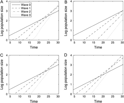
The size of the first four generations of cells. The log size of generations 1–4 is shown as a function of time t. Both time and space are plotted in units of $L = \log (1 / u)$ ⁠. (A) The average values of the log generation sizes over $10^{6}$ sample simulations. (B) The limiting approximation from Equation 3 for the log size of the generations. (C) The approximation from Equation 6 using the mean of $\log V_{d, k}$ ⁠. (D) The approximation from Equation 6 using a value two standard deviations above the mean of $\log V_{d, k}$ to demonstrate an extreme scenario. Parameters are $u = 10^{- 5}$ ⁠, $v \sim δ (b)$ ⁠, $a_{0} = 0.2$ ⁠, $b_{0} = 0.1$ ⁠, and $b = 0.05.$

Figure 4.—

Open in new tab Download slide

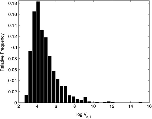
The distribution of log V_d,1. The relative frequency histogram of 1000 random samples from the distribution of $\log V_{d, 1}$ is shown, as specified by Equation 1.

TABLE 1

Means and standard deviations for log V_d,k for k = 1, 2, 3, as specified by Equation 1

Generation	Mean	Standard deviation
1	4.7638	1.3738
2	10.6010	2.2434
3	17.0519	3.0282

Open in new tab

TABLE 1

Means and standard deviations for log V_d,k for k = 1, 2, 3, as specified by Equation 1

Generation	Mean	Standard deviation
1	4.7638	1.3738
2	10.6010	2.2434
3	17.0519	3.0282

Open in new tab

While the limit in (3) depends on the fitness distribution only through the maximum attainable fitness increase b, the distribution of $V_{d, k}$ also depends on the fitness distribution through the probability of attaining a fitness advance of b if v is discrete and the value of the probability density function at b if v is continuous (see Equation 4.9 in Durrett et al. 2010). As a consequence, our finite time approximation (6) takes into consideration the shape of the fitness distribution near b and the corrector term log $V_{d, k}$ accounts for variations in the likelihood of attaining the maximum possible fitness advance.

Within-generation heterogeneity:

We begin our investigation of within-generation heterogeneity by examining the extent of diversity present in the first generation of cells. We use two statistical measures to assess heterogeneity: (i) Simpson's index, which is given by the probability that two randomly chosen cells from the first generation stem from the same clone, and (ii) the fraction of individuals in the first generation that stem from the largest family of cells. To obtain these results, we derive an alternate formulation of the limit in Equation 1 that shows the limit is the sum of points in a nonhomogeneous Poisson process (see the appendix for more details). Each point in the limiting process represents the contribution of a different mutant lineage to $Z_{1} (t)$ so that it suffices to calculate i and ii for the points in the limiting process.

Simpson's index:

Let us introduce some terminology by defining

X_{n}

to be the

n th

largest point in the limiting point process and by setting

S_{n} = \sum_{i = 1}^{n} X_{i}

⁠. Then Simpson's index for the point process is defined by

R = \frac{\sum_{i = 1}^{∞} X_{i}^{2}}{{(S_{∞})}^{2}} = {\sum_{i = 1}^{∞} (\frac{X_{i}}{S_{∞}})}^{2} .

We may also consider Simpson's index for a random walk

R_{n} = {\sum_{i = 1}^{n} (Y_{i} / W_{n})}^{2}

⁠, where the

Y_{i}

are independent random variables with a tail probability

P (Y_{i} > x) = x^{- α}

⁠, and

W_{n} = \sum_{i = 1}^{n} Y_{i}

⁠. Then the limit as n goes to infinity of

R_{n}

is

1 - α

(Fuchs et al. 2001), where

α = λ_{0} / λ_{1} \in (0, 1)

denotes the ratio of the growth rate of type-0 cells to the maximal growth rate of type-1 cells. Furthermore, the expected value of

R_{n}

converges to the expected value of R so we have

E R = 1 - α .

(7)

See the appendix for details of this calculation. Equation 7 shows that the average amount of heterogeneity present in the first generation depends only on α. Figure 5 displays the sample mean of Simpson's index of Z as a function of time for different values of α. Initially, the sample mean tends toward

1 - α,

the expected value of Simpson's index for the limiting point process. Although the sample mean is greater than the limiting value for larger values of b, our theory guarantees that eventually, the values of the sample mean converge. However, it is impossible to simulate the process for such long times since the population size and number of cell types become too large.

Figure 5.—

Open in new tab Download slide

The expected value of Simpson's index for the first wave of cells. The sample mean of Simpson's index (dots) over time t and the expected value of Simpson's index for the limiting point process (line) are shown, for two different values of $α$ ⁠. Parameters are $λ_{0} = 0.1$ ⁠, $a_{0} = 0.2$ ⁠, and $v \sim U ([0, b])$ ⁠, where $b = 0.01$ in a and $b = 0.05$ in b.

Expressions for the density and higher moments of R can be obtained in a similar manner by the comparison techniques we used in the proof of Equation 7 (see appendix and Logan et al. 1973; Shao 1997). In addition, near the origin, the density g(x) of R has the form

g (x) \sim a x^{- 3 / 2} \exp [- b x^{- 1}]

(8)

as

x \to 0

_. Figure 6 displays simulations of Simpson's index for the first wave mutants in the branching process Z. Note the convergence of the empirical distribution of Simpson's index to the distribution for the limiting point process.

Figure 6.—

Open in new tab Download slide

The empirical distribution of Simpson's index for the first wave of cells. Individual plots of Simpson's index are shown for the branching process at times $t = 70$ ⁠, 90, 110, and 130 along with Simpson's index for the limiting point process $(t = ∞)$ ⁠. The histograms show the average over 1000 sample simulations. For the limiting point process, we approximate Simpson's index by examining the largest $10^{4}$ points in the process. Parameters are $λ_{0} = 0.1$ ⁠, $a_{0} = 0.2$ ⁠, and $v \sim U ([0, 0.01])$ ⁠.

Largest clones:

To further investigate heterogeneity properties of the point process, we examine the fraction of cells descended from the largest family of first-generation mutants defined as $V_{n} = X_{1} / S_{n}$ ⁠. This quantity reveals the degree of dominance of the largest clone in the first wave of mutants. For large n, values of V_n near one indicate that the population is largely dominated by a single clone, while values near zero indicate a highly heterogeneous population where no single clone contributes significantly to the total. Using a similar approach to that in the previous section, we again consider this calculation in the context of a random walk. Consider a sequence of independent, identically distributed random variables Y_i with partial sums W_n. Define the maximum value of this sequence from 1 to n to be Y₍₁₎. Then classical results regarding one-dimensional random walks characterize the limiting characteristic function of W_n/Y₍₁₎ (Darling 1952). In the appendix, we demonstrate that these results can be applied to the study the largest clone contributions in the limiting point process.

We show that 1/V_n converges in distribution to a nontrivial limit W and obtain an explicit formula for the characteristic function of the limit: as

n \to ∞

⁠,

V_{n}^{- 1} \Rightarrow W

⁠, where W has characteristic function ψ satisfying ψ(0) = 1 and

ψ (t) = \frac{\exp [i t]}{f_{α} (t)} for all t \neq 0,

(9a)

with

f_{a} (t) = 1 + α \int_{0}^{1} (1 - e^{i t u}) u^{- (α + 1)} d u .

(9b)

Interestingly, the characteristic function of W is nonintegrable since its density has a singularity at 1. This finding implies that there is a disproportionately large chance that a single clone dominates the population. Further details are shown in the appendix.

Differentiating ψ then leads to simple expressions for the mean and variance of the limit,

E W = \frac{1}{1 - α} and var (W) = \frac{2}{{(1 - α)}^{2} (2 - α)} .

(10)

Figure 7a suggests that the rate of convergence is slow for α close to 1. These formulas provide us with the first two moments of the diversity measure W and reveal its dependence on α.

Figure 7.—

Open in new tab Download slide

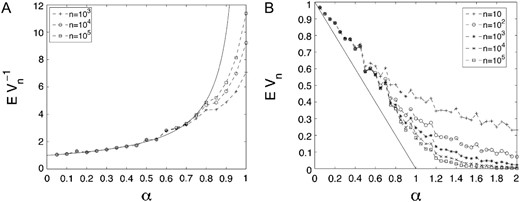
The largest clones in the population of cells. (A) A comparison between Monte Carlo estimates for $E V_{n}^{- 1}$ and the limit ${(1 - α)}^{- 1} .$ (B) A comparison of the Monte Carlo estimates for $E V_{n}$ and the curve ${(1 - α)}^{+}$ ⁠. The Monte Carlo estimates are averaged over 100 sample simulations.

Equation 9 implies that V_n converges to a nontrivial limit V = W⁻¹ and Jensen's inequality applied to the strictly convex function 1/x implies that $E (\lim X_{1} / S_{n}) > 1 - α .$ This result provides a lower bound on the expected value of the limit of V_n and indicates that for values of α close to zero, the population is eventually dominated by a single clone. Even though this result indicates only a lower bound, simulations suggest that deviations of the mean from 1−α are small, as illustrated in Figure 7b.

Extensions to generation k:

The results obtained in the previous two sections for the first generation of cells can easily be extended to later generations by noting that each mutation to a type-(k − 1) individual starts a new family regardless of the mutated cell's family tree. Therefore, the amount of heterogeneity within generation k depends on the relative growth rates of type-k and type-(k − 1) individuals in the same way that the amount of heterogeneity within generation 1 depends on the relative growth rates of type-1 and type-0 individuals. In particular, letting R_k denote the limiting value of Simpson's index for generation k, we have

E R_{k} = 1 - α_{k},

(11)

where

α_{k} = λ_{k - 1} / λ_{k}

is the relative growth rate of type-(k −1) individuals compared to type-k individuals (see also Equation 7 above). Note that the relative growth rates α_k are increasing functions of k. Therefore, Equation 11 shows that the mean of Simpson's index is a decreasing function of the generation number.

Total population heterogeneity:

We conclude this section by demonstrating how heterogeneity measures for the population as a whole can be calculated using information about both intra- and interwave heterogeneity. First, define the total collection of all genotypes present at time t as N(t). For a particular genotype, x, the number of cells at time t that have exactly this genotype is given by Z^(x)(t). Two cells have the same genotype if they contain exactly the same collection of mutations. Then Simpson's index for the entire population is given by

SI (Z (t)) = \sum_{x \in N (t)} {(\frac{Z^{(x)} (t)}{Z (t)})}^{2} .

To show how this expression depends on the contributions of different waves, define the total collection of genotypes present in the wave-k population at time t by N_k(t), and let Z_k^(x) be the population of cells in wave k that have genotype x. By defining K(t) to be the number of waves present at time t, we obtain the alternate expression

SI (Z (t)) = {\sum_{k = 0}^{K (t)} \sum_{x_{k} \in N_{k} (t)} (\frac{Z_{k}^{(x_{k})} (t)}{Z_{k} (t)})}^{2} {(\frac{Z_{k} (t)}{Z (t)})}^{2} .

This decomposition expresses Simpson's index for the whole population in terms of Simpson's index for each wave and the contribution of each wave to the total population. Combining the result in (5), which gives the dominant wave as a function of time, with (11), which describes wave-k heterogeneity, we obtain a description of how the extent of heterogeneity changes in time. However, more refined results are needed to describe the transitions between the dominance of successive waves.

DISCUSSION

In this article, we investigated the evolution of intratumor heterogeneity in a stochastic model of tumor cell expansion. Our model incorporates random mutational advances conferred by (epi)genetic alterations and our analysis focused on the extent of heterogeneity present in the tumor. We first considered heterogeneity between tumor subpopulations with varying numbers of alterations and obtained limiting results, as the mutation rate approaches zero, for the contribution of each wave of mutants to the total tumor cell population. We showed that in the limit, this intergeneration heterogeneity depends on the maximum attainable fitness advance conferred by (epi)genetic alterations, but not on the specific form of the mutational fitness distribution. Our analysis also led to analytical expressions for the arrival time of the first cell with k mutations and showed that the rate of accumulation of new genetic alterations accelerates over time due to the increasing growth rates of successive generations. We demonstrated with stochastic simulations that for small but positive mutation rates, our limiting approximations provide good predictions of the model behavior (see Figure 3). These simulations also suggest that as time increases, multiple waves of mutants coexist without a single, largely dominant wave. For large t, the mean growth rate of the kth wave is given by $λ_{0} + k b$ ⁠, showing that variation in fitness within a particular wave is a transient property. The extent to which this variation affects tumor dynamics at small times is the subject of ongoing work.

We also investigated the genotypic diversity present within the kth generation of mutants by considering two measures of diversity: Simpson's index, which is given by the probability that two randomly selected cells stem from the same family, and the fraction of individuals in generation k that stem from the largest family of individuals. We obtained limiting expressions for the mean of Simpson's index as well as the form of its density near the origin. Interestingly, the limiting mean of Simpson's index is given by the quantity 1−α, where α is the ratio between the maximum attainable fitness values of type-(k − 1) and type-k individuals. We then observed that, as time increases, the mass of the distribution of Simpson's index moves closer to 0, indicating higher levels of diversity in the tumor at later times (see Figure 6). This behavior was also observed via direct numerical simulation of the branching process—the distribution and mean of Simpson's index converged to the predicted limiting values.

Finally, we investigated the ratio between the total population size of the kth wave of mutants and the size of the largest family. We showed that this ratio can be approximated by a random variable with mean (1−α)⁻¹. An explicit formula for the characteristic function of this random variable was also obtained (see Equation 9). Note that as α approaches 1, the mean of the ratio grows to infinity—i.e., the largest family of cells constitutes a vanishing proportion of the total population of wave-k cells as the maximum possible fitness advance goes to zero.

In the context of tumorigenesis, where a tumor originally starting from a single cell reaches cell numbers of ≥10¹², the limit as t goes to infinity is indeed the appropriate regime of study. We have compared our results regarding Simpson's index with numerical simulations at finite times (see, e.g., Figures 5 and 6) and have found good qualitative agreement with the asymptotic limits. Estimates of overall mutation rates in evolving cancer cell populations range from 10⁻⁹ to 10⁻². In Figure 3 we demonstrate good agreement between our results regarding interwave heterogeneity in the small mutation rate limit $(u \to 0)$ and numerical simulations when the mutation rate is $10^{- 5}$ ⁠; thus, analysis in this limiting regime captures the dynamics for mutation rates < $10^{- 5}$ per cell division.

In conclusion, our analysis indicates that tumor diversity is strongly dependent upon the age of the tumor and the maximum attainable fitness advance of mutant cells. If only small fitness advances are possible, then the tumor population is expected to have a larger extent of diversity compared to situations in which fitness advances are large. The acceleration of waves observed in our studies of intergeneration heterogeneity provides evidence that an older tumor has a higher level of diversity than a young tumor. In addition, we have shown that the mean of Simpson's index for generation k is a decreasing function of the generation number (see Equation 11), indicating a larger extent of diversity in later generations and suggesting a further increase in the total extent of heterogeneity present in the tumor at later times.

Possible extensions of our model include spatial considerations and the effects of tissue organization on the generation of intratumor heterogeneity as well as the inclusion of other cell types, such as immune system cells and the microenvironment. Furthermore, alternative growth dynamics should be considered to test the extent of heterogeneity arising in populations that follow logistic, Gompertzian, or other growth models. We have neglected these aspects in the current version of the model to focus on the dynamics of tumor diversity in an exponentially growing population of cells. Our model provides a rational understanding of the extent and dynamics of intratumor heterogeneity and is useful for obtaining an accurate picture of its generation during tumorigenesis.

Acknowledgements

The authors thank Theresa Edmonds for exceptional research assistance. This work is supported by National Cancer Institute grant U54CA143798 (to J.F., K.L., and F.M.), National Science Foundation (NSF) grant DMS 0704996 (to R.D.), and NSF RTG grant DMS 0739164 (to J.M.).

Footnotes

Communicating editor: M. W. Feldman

LITERATURE CITED

Beerenwinkel

N

,

Antal

T

,

Dingli

D

,

Traulsen

A

,

Kinzler

K W

et al. ,

2007

Genetic progression and the waiting time to cancer

.

PLoS Comput. Biol.

3

:

e225

.

Bozic

I

,

Antal

T

,

Ohtsuki

H

,

Carter

H

,

Kim

D

et al. ,

2010

Accumulation of driver and passenger mutations during tumor progression

.

Proc. Natl. Acad. Sci. USA

107

:

18545

–

18550

.

Google Scholar

Crossref

WorldCat

Campbell

L L

,

Polyak

K

,

2007

Breast tumor heterogeneity: Cancer stem cells or clonal evolution?

Cell Cycle

6

:

2332

–

2338

.

Coldman

A J

,

Goldie

J H

,

1985

Role of mathematical modeling in protocol formulation in cancer chemotherapy

.

Cancer Treat. Rep.

69

:

1041

–

1048

.

Google Scholar

PubMed

OpenURL Placeholder Text

WorldCat

Coldman

A J

,

Goldie

J H

,

1986

A stochastic model for the origin and treatment of tumors containing drug-resistant cells

.

Bull. Math. Biol.

48

:

279

–

292

.

Darling

D A

,

1952

The role of the maximum term in the sum of independent random variables

.

Trans. Am. Math. Soc.

72

:

85

–

107

.

Google Scholar

OpenURL Placeholder Text

WorldCat

Dick

J E

,

2008

Stem cell concepts renew cancer research

.

Blood

112

:

4793

–

4807

.

Durrett

R

,

2005

Probability: Theory and Examples

.

Brooks Cole–Thomson Learning

,

Belmont, CA

.

Google Scholar

Google Preview

OpenURL Placeholder Text

WorldCat

Durrett

R

,

Moseley

S

,

2010

Evolution of resistance and progression to disease during clonal expansion of cancer

.

Theor. Popul. Biol.

77

:

42

–

48

.

Durrett

R

,

Foo

J

,

Leder

K

,

Mayberry

J

,

Michor

F

,

2010

Evolutionary dynamics of tumor progression with random fitness values

.

Theor. Popul. Biol.

78

:

54

–

66

.

Durrett

R

,

Mayberry

J

,

2011

Traveling waves of selective sweeps

.

Ann. Appl. Probab.

21

:

699

–

744

.

Google Scholar

Crossref

WorldCat

Durrett

R

,

Moseley

S

,

2010

Evolution of resistance and progression to disease during clonal expansion of cancer

.

Theor. Popul. Biol.

77

:

42

–

48

.

Durrett

R

,

Foo

J

,

Leder

K

,

Mayberry

J

,

Michor

F

,

2010

Evolutionary dynamics of tumor progression with random fitness values

.

Theor. Popul. Biol.

78

:

54

–

66

.

Fidler

I J

,

1978

Tumor heterogeneity and the biology of cancer invasion and metastasis

.

Cancer Res.

38

:

2651

–

2660

.

Google Scholar

PubMed

OpenURL Placeholder Text

WorldCat

Fidler

I J

,

Hart

I R

,

1982

Biological diversity in metastatic neoplasms: origins and implications

.

Science

217

:

998

–

1003

.

Foley

M

,

Tilley

L

,

1997

Quinoline antimalarials: mechanisms of action and resistance

.

Int. J. Parasitol.

27

:

231

–

240

.

Fuchs

A

,

Joffe

A

,

Teugels

J

,

2001

Expectation of the ratio of the sum of squares to the square of the sum: exact and asymptotic results

.

Theory Probab. Appl.

46

:

243

–

255

.

Google Scholar

Crossref

WorldCat

Geisler

J P

,

Rose

S L

,

Geisler

H E

,

Miller

G A

,

Wiemann

M C

,

2002

Drug resistance and tumor heterogeneity

.

CME J. Gynecol. Oncol.

7

:

25

–

28

.

Google Scholar

OpenURL Placeholder Text

WorldCat

Gerrish

P J

,

Lenski

R E

,

1998

The fate of competing beneficial mutations in an asexual population

.

Genetica

102–103

:

127

–

144

.

Google Scholar

PubMed

OpenURL Placeholder Text

WorldCat

Haeno

H

,

Iwasa

Y

,

Michor

F

,

2007

The evolution of two mutations during clonal expansion

.

Genetics

177

:

2209

–

2221

.

Haggarth

L

,

Auer

G

,

Busch

C

,

Norberg

M

,

Haggman

M

et al. ,

2005

The significance of tumor heterogeneity for prediction of DNA ploidy of prostate cancer

.

Scand. J. Urol. Nephrol.

39

:

387

–

392

.

Heppner

G H

,

1984

Tumor heterogeneity

.

Cancer Res.

44

:

2259

–

2265

.

Google Scholar

PubMed

OpenURL Placeholder Text

WorldCat

Imhof

M

,

Schlotterer

C

,

2001

Fitness effects of advantageous mutations in evolving Escherichia coli populations

.

Proc. Natl. Acad. Sci. USA

98

:

1113

–

1117

.

Google Scholar

Crossref

WorldCat

Kansal

A R

,

Torquato

S

,

Chiocca

E A

,

Deisboeck

T S

,

2000

Emergence of a subpopulation in a computational model of tumor growth

.

J. Theor. Biol.

207

:

431

–

441

.

Komarova

N

,

2006

Stochastic modeling of drug resistance in cancer

.

J. Theor. Biol.

239

:

351

–

366

.

Kunkel

T A

,

Bebenek

K

,

2000

DNA replication fidelity

.

Annu. Rev. Biochem.

69

:

497

–

529

.

Lai

L A

,

Paulson

T G

,

Li

X

,

Sanchez

C A

,

Maley

C

et al. ,

2007

Increasing genomic instability during premalignant neoplastic progression revealed through high resolution array-CGH

.

Genes Chromosomes Cancer

46

:

532

–

542

.

Lenski

R E

,

Travisano

M

,

1994

Dynamics of adaptation and diversification: a 10,000-generation experiment with bacterial populations

.

Proc. Natl. Acad. Sci. USA

91

:

6808

–

6814

.

Google Scholar

Crossref

WorldCat

Lenski

R E

,

Rose

M R

,

Simpson

S C

,

Tadler

S C

,

1991

Long-term experimental evolution in Escherichia coli. I. Adaptation and divergence during 2,000 generations

.

Am. Nat.

138

:

1315

–

1341

.

Google Scholar

Crossref

WorldCat

Logan

B F

,

Mallows

C L

,

Rice

S O

,

Shepp

L A

,

1973

Limit distributions of self-normalized sums

.

Ann. Probab.

1

:

788

–

809

.

Google Scholar

Crossref

WorldCat

Loya

P

,

2005

Dirichlet and fresnel integrals via integrated integration

.

Math. Mag.

78

(

1

):

63

–

67

.

Google Scholar

Crossref

WorldCat

Maley

C C

,

Galipeau

P C

,

Finley

J C

,

Wongsurawat

V J

,

Li

X

et al. ,

2006

Genetic clonal diversity predicts progression to esophageal adenocarcinoma

.

Nat. Genet.

38

:

468

–

473

.

Merlo

L M

,

Pepper

J W

,

Reid

B J

,

Maley

C C

,

2006

Cancer as an evolutionary and ecological process

.

Nat. Rev. Cancer

6

:

924

–

935

.

Michelson

S

,

Ito

K

,

Tran

H T

,

Leith

J T

,

1989

Stochastic models for subpopulation emergence in heterogeneous tumors

.

Bull. Math. Biol.

51

:

731

–

747

.

Nguyen

H N

,

Sevin

B U

,

Averette

H E

,

Ramos

R

,

Ganjei

P

et al. ,

1993

Evidence of tumor heterogeneity in cervical cancers and lymph node metastases as determined by flow cytometry

.

Cancer

71

:

2543

–

2550

.

Nicolson

G L

,

1984

Generation of phenotypic diversity and progression in metastatic tumor cells

.

Cancer Metastasis Rev.

3

:

25

–

42

.

Oller

A R

,

Rastogi

P

,

Morgenthaler

S

,

Thilly

W G

,

1989

A statistical model to estimate variance in long term-low dose mutation assays: testing of the model in a human lymphoblastoid mutation assay

.

Mutat. Res.

216

:

149

–

161

.

O'Sullivan

M

,

Budhraja

V

,

Sadovsky

Y

,

Pfeifer

J D

,

2005

Tumor heterogeneity affects the precision of microarray analysis

.

Diagn. Mol. Pathol.

14

:

65

–

71

.

Park

S C

,

Krug

J

,

2007

Clonal interference in large populations

.

Proc. Natl. Acad. Sci. USA

104

:

18135

–

18140

.

Google Scholar

Crossref

WorldCat

Park

S C

,

Simon

A

,

Krug

J

,

2010

The speed of evolution in large asexual populations

.

J. Stat. Phys.

138

:

381

–

410

.

Google Scholar

Crossref

WorldCat

Resnick

S

,

1987

Extreme Values, Regular Variation, and Point Processes

.

Springer-Verlag

,

Berlin/Heidelberg, Germany/New York

Ridout

M S

,

2008

Generating random numbers from a distribution specified by its laplace transform

.

Stat. Comput.

19

:

439

–

450

.

Google Scholar

Crossref

WorldCat

Rokyta

D R

,

Beisel

C J

,

Joyce

P

,

Ferris

M T

,

Burch

C L

et al. ,

2008

Beneficial fitness effects are not exponential for two viruses

.

J. Mol. Evol.

67

:

368

–

376

.

Sanjuan

R

,

Moya

A

,

Elena

S F

,

2004

The distribution of fitness effects caused by single-nucleotide substitutions in an RNA virus

.

Proc. Natl. Acad. Sci. USA

101

:

8396

–

8401

.

Google Scholar

Crossref

WorldCat

Schweinsberg

J

,

2008

The waiting time for m mutations. Electron

.

J. Probab.

13

:

1442

–

1478

.

Google Scholar

OpenURL Placeholder Text

WorldCat

Seshadri

R

,

Kutlaca

R J

,

Trainor

K

,

Matthews

C

,

Morley

A A

,

1987

Mutation rate of normal and malignant human lymphocytes

.

Cancer Res.

47

:

407

–

409

.

Google Scholar

PubMed

OpenURL Placeholder Text

WorldCat

Shao

Q M

,

1997

Self-normalized large deviations

.

Ann. Probab.

25

:

285

–

328

.

Google Scholar

Crossref

WorldCat

Shipitsin

M

,

Campbell

L L

,

Argani

P

,

Weremowicz

S

,

Bloushtain-Qimron

N

et al. ,

2007

Molecular definition of breast tumor heterogeneity

.

Cancer Cell

11

:

259

–

273

.

Wolman

S R

,

1986

Cytogenetic heterogeneity: its role in tumor evolution

.

Cancer Genet. Cytogenet.

19

:

129

–

140

.

APPENDIX

Convergence in distribution of Z_k(t):

Define λ_k = λ₀ + kb to be the maximum growth rate that can be attained by a generation k mutant, and let

p_{k} = - k + \overset{k - 1}{\sum_{j = 0}} \frac{λ_{k}}{λ_{j}} .

If ν is discrete and assigns mass g_i to a finite number of values b₁ < b₂ < … <b_N = b, then

{(1 / u)}^{k + p_{k}} e^{- λ_{k} t} Z_{k} (t) \Rightarrow V_{d, k},

(A1)

where “⇒” denotes convergences in distribution, and V_d,k has Laplace transform

\exp [- d_{k} (λ_{0}, b) V_{0} θ^{λ_{0} / λ_{k}}]

for all θ ≥ 0.

If instead ν is a continuous distribution on [0, b] with a bounded density g that is continuous and positive at b, then

{(t / u)}^{k + p_{k}} e^{- λ_{k} t} Z_{k} (t) \Rightarrow V_{c, k},

(A2)

where V_c,k has Laplace transform

\exp [- c_{k} (λ_{0}, b) V_{0} θ^{λ_{0} / λ_{k}}]

for all θ ≥ 0. Here d_k(λ₀, b) and c_k(λ₀, b) are constants that depend on the model parameters (Durrett et al. 2010), and “d” and “c” in the constants and subscripts stand for discrete and continuous. See Durrett and Moseley (2010) for a proof of Equation A1 and Durrett et al. (2010) for a proof of (A2). To show the dependence on the density g, we write the value of c₁(λ₀, b) as

c_{1} (λ_{0}, b) = g (b) \frac{λ_{0} + b}{λ_{0}} \cdot \frac{1}{λ_{0} + b} {(\frac{a_{0} + b}{λ_{0} + b})}^{- b / (λ_{0} + b)} Γ (\frac{λ_{0}}{λ_{0} + b}) Γ (1 - \frac{λ_{0}}{λ_{0} + b}) .

The convergence in (A2) was also numerically investigated in Figures 1 and 2 of Durrett et al. (2010).

Point process limit:

In this section, we discuss the point process representation for the limit in Equations A1 and A2 in the case where k = 1. The limit is the sum of points in a nonhomogeneous Poisson process. Before stating this result, we introduce some terminology. Here and in what follows, we use $| A |$ to denote the number of points in the set A. We say that Λ is a Poisson process on (0, ∞) with mean measure μ if Λ is a random set of points in (0, ∞) with the following properties:

For any A⊂(0, ∞), N(A) = $| Λ \cap A |$ is a Poisson random variable with mean μ(A).
For any k ≥ 1, if A₁, … , A_k are disjoint subsets of (0, ∞), then N(A_i), 1 ≤ i ≤ k are independent.

We also let α = λ₀/λ₁ ∈ (0, 1) denote the ratio of the growth rate of type-0 cells to the maximal growth rate of type-1 cells and note that 1 + p₁ = 1/α.

Theorem 1. Let Λ be a Poisson process on (0, ∞) with mean measure

μ (A) = \int_{A} α z^{- (α + 1)} d z

and let S denote the sum of the points in Λ. Then positive constants A_d, A_c = A_d(λ₀, b), A_c(λ₀, b) exist that depend on the indicated parameters so that in case i as t →∞

{(A_{d} u V_{0})}^{- (1 + p_{1})} e^{- λ_{1} t} Z_{1} (t) \Rightarrow S,

and in case ii as t →∞

{(A_{c} u V_{0})}^{- (1 + p_{1})} t^{1 + p_{1}} e^{- λ_{1} t} Z_{1} (t) \Rightarrow S .

For more details, see Durrett et al. (2010), Theorem 3, and Durrett and Moseley (2010), Corollary to Theorem 3. Note that the mean measure for Λ has tail m(x, ∞) = x^−α.

Let X_n denote the nth largest point in Λ, and let

S_{n} = \sum_{i = 1}^{n} X_{i}

denote the sum of the n largest points. To determine the dependence of X_n on n we first note that if we define Λ′ = f (Λ) where f (x) = x^−α, then Λ′ is a Poisson process and after making the change of variables y = x^−α, we can see that the mean measure is

μ' (A) = \int_{f^{- 1} (A)} α x^{- (α + 1)} d x = \int_{A} d y = | A | .

In other words, Λ′ is a homogeneous Poisson process with constant intensity and hence the spacings between points are independent exponentials with mean 1. If we let T_n denote the time of the nth arrival in Λ′, then the law of large numbers implies that T_n ∼ n as n → ∞. Since

X_{n} = T_{n}^{- 1 / α}

⁠, we obtain X_n ∼ n^−1/α as n → ∞. In addition, we have the following Lemma:

Lemma 1.

E X_{n} = \frac{Γ (n - 1 / α)}{Γ (n)} .

Furthermore, if we define

S_{∞} = \sum_{i =1}^{∞} X_{i}

⁠, then

E S_{∞} < ∞ .

Proof. Since T_n has a Gamma(n, 1) distribution, we have $E X_{n} = E T_{n}^{- 1 / α} = Γ (n - 1 / α) / Γ (n) .$ Stirling's approximation implies that Γ(n − 1/α)/ Γ(n) ∼ n^−1/α and the second conclusion follows. ■

Simpson's index:

To prove Equation 7 in the text, we use a result in Fuchs et al. (2001) that shows that

\lim_{n \to \infty} E R_{n} = 1 - α .

(A3)

Here

R_{n} = \overset{n}{\sum_{i = 1}} {(\frac{Y_{i}}{S_{n}})}^{2},

where Y_i are iid random variables in the domain of attraction of a stable law with index α and S_n = Y₁ + … + Y_n. To explain the connection between the two results, note that if we have P(Y_i > x) = x^−α, for x ≥ 1 and letting Y_n_,i = Y_i/n^1/α, then

n P (Y_{n, i} \in A) \to μ (A) .

This implies that if we let Δ_n = {Y_n_,i : i ≤ n} be the point process associated with the Y_n_,i and define the measures

ξ_{n} \equiv \sum_{x \in Λ_{n}} δ_{x}

and

ξ = \sum_{x \in Λ} δ_{x},

then we have

ξ_{n} \Rightarrow ξ,

so that we should expect ER to agree with lim ER_n.

To make this argument rigorous, let

R_{n} (ε) = \frac{\sum_{i = 1}^{n} Y_{n, i}^{2} 1_{Y_{n, i} > ε}}{{(\sum_{i = 1}^{n} Y_{n, i}^{2} 1_{Y_{n, i} > ε})}^{2}}

denote the truncated value of Simpson's index for Λ_n and

R (ε) = \frac{\sum_{i}^{\infty} X_{i}^{2} 1_{X_{i} > ε}}{{(\sum_{i = 1}^{\infty} X_{i} 1_{X_{i} > ε})}^{2}}

denote the truncated value for Λ. Then for any ε > 0, we have

| E R_{n} - E R | \leq E | R_{n} - R_{n} (ε) | + E | R_{n} (ε) - R (ε) | + E | R (ε) - R | .

(A4)

We complete the proof by deriving appropriate bounds for each of the three terms on the right-hand side of (A4). For the first term, we have the following:Lemma 2.

\lim_{n \to \infty} \sup E | R_{n} - R_{n} (ε) | \leq h_{ε},

where h_ε → 0 as ε → 0.

Proof. Let ε > 0 and write

A_{n, k} = \sum_{i = 1}^{n} Y_{n, i}^{k},

A_{n, k} (ε) = \sum_{i = 1}^{n} Y_{n, i}^{k} 1_{Y_{n, i} > ε},

and

{\bar{A}}_{n, k} (ε) = A_{n, k} - A_{n, k} (ε)

for k = 1, 2. Since

E Y_{1}^{k} 1_{Y_{1} \leq ε n^{1 / α}} = \int_{1}^{ε n^{1 / α}} k y^{k - 1} y^{- α} d y \leq C ε^{k - α} n^{k / α - 1}

for k = 1, 2, we have the bound

E {\bar{A}}_{n, k} (ε) \leq C ε^{k - α} .

(A5)

After noting that

A_{n, 2} \leq A_{n, 1}^{2},

A_{n, 2} (ε) \leq A_{n, 1}^{2} (ε) \leq A_{n, 1}^{2},

and

{\bar{A}}_{n, 1} (ε) + A_{n, 1} (ε) = A_{n, 1},

we have for any δ > 0,

\begin{array}{l} E | R_{n} - R_{n} (ε) | = E | \frac{{\bar{A}}_{n, 2} (ε)}{A_{n, 1}^{2}} + R_{n} (ε) (\frac{A_{n, 1}^{2} (ε) - A_{n, 1}^{2}}{A_{n, 1}^{2}}) | \\ \leq δ^{- 2} E {\bar{A}}_{n, 2} (ε) + P (A_{n, 1} \leq δ) \\ + δ^{- 1} E (\frac{| 2 A_{n, 1} (ε) {\bar{A}}_{n, 1} (ε) {\bar{A}}_{n, 1}^{2} (ε) |}{A_{n, 1}}) + P (A_{n, 1} \leq δ) \\ = δ^{- 2} E | {\bar{A}}_{n, 2} (ε) | + δ^{- 1} E (| {\bar{A}}_{n, 1} (ε) (2 + \frac{A_{n, 1} (ε)}{A_{n, 1}}) |) + 2 P (A_{n, 1} \leq δ) \\ \leq δ^{- 2} E {\bar{A}}_{n, 2} (ε) + 3 δ^{- 1} E {\bar{A}}_{n, 1} (ε) + 2 P (A_{n, 1} \leq δ) \\ \leq \frac{ε^{2 - α}}{δ^{2}} + \frac{3 ε^{1 - α}}{δ} + 2 P (A_{n, 1} \leq δ), \end{array}

(A6)

where we have used (A5) in the last line. To control the third term on the right, let φ denote the Laplace transform of Y₁. Then

\begin{matrix} 1 - φ (t) = α \int_{1}^{\infty} (1 - e^{- t y}) y^{- (α + 1)} d y \\ = α t^{α} \int_{t}^{∞} (1 - e^{- x}) x^{- (α + 1)} d x \sim C t^{α} \end{matrix}

as t → 0 since 1 − e^−x ∼ x as x → 0 implies that

\int_{0}^{\infty} (1 - e^{- x}) x^{- (α + 1)} d x < ∞ .

We can conclude that

E \exp (- t A_{n, 1}) = (1 - {(1 - φ \frac{t}{n^{1 / α}})}^{n}) \to \exp (- C t^{α})

as n → ∞. In particular, A_n,₁ ⇒ A₁, where A₁ has the above Laplace transform. Since

1 - \exp (- C t^{α}) \to 1

as t → ∞, we have P(A₁ = 0) = 0 so that taking δ = ε^(1−α)/2 in (A6) yields the result. ■

To bound the second term on the right-hand side of (A4), we need some notation. Let M_p denote the class of all point measures on (0, ∞). In a slight abuse of notation, we write v ∈ ν when ν ∈ M_p and v ∈ supp(ν). We equip M_p with the topology of vague convergence (see, for example, Section 3.4 in Resnick 1987) and take as our σ-algebra the one generated by open sets in this topology. Associated with any random set of points, we can associate a measure ξ that is a random variable with values in M_p_. We write Λ_n ⇒ Λ to mean that the associated random measures ξ_n ⇒ ξ.Lemma 3. Λ_n ⇒ Λ and if we define the maps F_k_,ε: M_p → [0, ∞) by

F_{k, ε} (μ_{n}) = \sum_{x \in μ_{n}} x^{k} 1_{x > ε}

for k = 1, 2, then

(F_{1, ε} (Λ_{n}), F_{2, ε} (Λ_{n})) \Rightarrow (F_{1, ε} (Λ), F_{2, ε} (Λ)) .

Proof.Since

n P (Y_{n, i} \in A) = n \int_{n^{1 / α} A} α y^{- (α + 1)} d y = \int_{A} α x^{- (α + 1)} d x = μ (A)

for all Borel sets A, the first claim follows from Proposition 3.21 in Resnick (1987). The second claim follows from the continuous mapping theorem (see, for example, Resnick 1987, p. 152) the fact that F_k_,ε is continuous away from measures ν with ε ∉ ν and the fact that the random measure associated with Λ has no point masses with probability 1. ■

As a consequence of this lemma, the fact that R_n(ε) ≤ 1, and the bounded convergence theorem, we have the following:

Corollary 1.

E | R_{n} (ε) - R (ε) | \to 0

as n → ∞ for any ε > 0.

It thus remains to establish the following:

Lemma 4.

\lim_{ε \to 0} \sup E | R (ε) - R | = 0.

Proof. We can establish this result using the same results as in the proof of Lemma 2, in particular if we define

A_{k} = \sum_{n = 1}^{∞} X_{n}^{k}

and

{\bar{A}}_{k} (ε) = \sum_{n = 1}^{∞} X_{n}^{k} 1_{X_{n} <εE}

for k = 1, 2. Then, following the display in Equation A6, we have for any δ > 0

E | R - R (ε) | \leq δ^{- 2} E {\bar{A}}_{2} (ε) + 3 δ^{- 1} E {\bar{A}}_{1} (ε) + 2 P (A_{1} \geq δ) .

It is obvious that P(A₁ = 0) = 0 and

E {\bar{A}}_{2} (ε) \leq E {\bar{A}}_{1} (ε)

for ε < 1, so it remains only to establish that

E {\bar{A}}_{1} (ε) \to 0,

as ε → 0. This result follows immediately from Lemma 1. Therefore, taking

δ = {(E {\bar{A}}_{1} (ε))}^{1 / 4}

completes the proof. ■

We can now complete the proof of Equation 7 by letting n → ∞ and then ε → 0 in (A4) and applying Lemmas 2 and 4 and Corollary 1.

To prove Equation 8, we use a result in Logan et al. (1973) that establishes that as n → ∞,

S_{n} (2) = R^{- 1 / 2} = \frac{\sum_{i = 1}^{n} Y_{i}}{{(\sum_{i = 1}^{n} Y_{i}^{2})}^{1 / 2}}

has a limiting distribution with a density f that satisfies

f (y) \sim a e^{- b y^{2}}, as y \to \infty,

for some constants a, b > 0 (see Logan et al. 1973, Equation 5.7, and Shao 1997, Theorem 6.1). Making the change of variables x = y^−1/2 yields Equation 8. ■

Largest clones:

Equation 9 is a consequence of the following theorem:Theorem 2. As n → ∞,

V_{n}^{- 1} \Rightarrow W,

where W has characteristic function ψ satisfying ψ (0) = 1 and

ψ (t) = \frac{e^{i t}}{f_{α} (t)}

for all t ≠ 0 with

f_{α} (t) = 1 + α \int_{0}^{1} (1 - e^{i t u}) u^{- (α + 1)} d u .

The form of the characteristic function is the same as the characteristic function for lim_n_→∞T_n/Y₍₁₎, where the Y_i are iid random variables with power law tails, Y₍₁₎ = max_i_≤nY_i, and $T_{n} = \sum_{i = 1}^{n} Y_{i}$ (see, for example, Darling 1952). Again, this agreement is a consequence of the previously discussed connection between Δ_n and the limiting Poisson point process.

To prove Theorem 2, we need the following notation. For a real number t, we define the function

s g n (t) = {\begin{cases} - 1, t < 0 \\ 0, t = 0 \\ 1, t > 0. \end{cases}

For a complex number z we denote the real part of z by Re[z] and its imaginary part by Im[z].

Proof of Theorem 2. Theorem 5.1 in Darling (1952) implies that we have

E \exp (i t T_{n} / Y_{(1)}) \to ψ (t)

as n → ∞ whereas in the Simpson's index section, Y₍₁₎ = max_i_≤nY_i and

T_{n} = \sum_{i = 1}^{n} Y_{i} .

To conclude that T_n/Y₍₁₎ ⇒ V, we need to show that y is continuous at 0. To establish this fact, we make the change of variables v = tu to conclude that

f_{α} (t) = 1 + α \int_{0}^{1} (1 - e^{i t u}) u^{- (α + 1)} d u = 1 + α {| t |}^{α} \int_{0}^{| t |} (1 - e^{i v sgn (t)}) v^{- (α + 1)} d v .

(A7)

Since 1 − exp(iv) ∼ −iv as v → 0, the integral on the right-hand side of (A7) is finite and hence

ψ (t) = e^{i t} f_{α}^{- 1} (t) \to 1

as t → 0. Since T_n/Y₍₁₎ ⇒ V, the fact that S_n/X₁ ⇒ V follows from the arguments in the previous section. ■

It is interesting to note that the characteristic function in Theorem 2 is not integrable. The problem is that the density of

V_{n}^{- 1}

blows up near 1. As an explanation for this, we note that with probability

\exp (- (1 - x^{- α})) \exp (- x^{- α}) x^{- α} = e^{- 1} x^{- α}

there is a point in the process bigger than x and no points in [1, x). When this happens,

V_{n}^{- 1} = \frac{S_{n}}{X_{1}} \leq 1 + \frac{n}{x}

and so

F_{n} (y) = P (V_{n}^{- 1} \leq y) \geq e^{- 1} n^{- α} {(y - 1)}^{α} .

If we had F_n(y) ? (y − 1)^α, then the density would blow up like (y−1)^α−1 as y → 1. We confirm that this gives the right asymptotic by providing an explicit formula for the density of W.

Corollary 2. W has a density on (1, ∞) given by

f (y) = \lim_{M \to ∞} \int_{- M}^{M} \frac{e^{i t (1 - y)}}{f_{α} (t)} d t .

Note that integral expression above does not converge absolutely so part of the proof consists of showing that the limit exists. If we apply the change of variable s = t(y − 1) in the definition of f, we see that

f (y) = {(y - 1)}^{α - 1} \int_{- ∞}^{∞} \frac{e^{- i t}}{{(y - 1)}^{α} + \int_{0}^{{(y - 1)}^{- 1}} ((1 - e^{i u t}) / u^{α + 1)}) d u},

thus confirming the intuition that the density blows up like (y − 1)^α⁻¹ as y approaches 1.

Proof of Corollary 2. We first establish that there are no point masses in the distribution of V. By the inversion formula we have for any a ∈ ℝ,

\begin{matrix} P (V = a) = \lim_{T \to ∞} \frac{1}{2 T} \int_{- T}^{T} e^{- i a t} ψ (t) d t \\ = \lim_{T \to ∞} \frac{1}{2 T} \int_{- T}^{T} \frac{e^{i t (1 - a)}}{f_{α} (t)} d t . \end{matrix}

If we focus on the positive axis and use the change of variable s = t/T,

\frac{1}{2 T} \int_{0}^{T} \frac{e^{i t (1 - a)}}{f_{α} (t)} d t = \frac{1}{2} \int_{0}^{1} \frac{e^{i s T (1 - a)}}{f_{α} (s T)} d s .

From display (A7) it follows that for every s ∈ (0, 1) we have e^isT^(1−a)/f_α(sT) → 0 as T→∞. Note that

R e [f_{α} (t)] = 1 + α \int_{0}^{1} \frac{1 - \cos u t}{u^{α + 1}} d u > 1,

which implies |f_α(t)| ≥ 1 for all t. Therefore |e^isT^(1−a)/f_α(t)| ≤ 1 for all t and it follows via the dominated convergence theorem that

\lim_{T \to ∞} \frac{1}{2} \int_{0}^{1} \frac{e^{i s T (1 - a)}}{f_{α} (s T)} d s = 0.

A similar result holds for the integral on the negative axis and we conclude that

P (V = a) = 0.

We can therefore conclude for x > 1 and h > 0 via the inversion formula (see Durrett 2005, Equation 3.2) and Fubini's theorem that

\begin{matrix} P (V \in (x, x + h)) = \lim_{T \to ∞} \frac{1}{2 π} \int_{- T}^{T} \int_{x}^{x + h} e^{- i t y} ψ (t) d y d t \\ = \lim_{T \to ∞} \frac{1}{2 π} \int_{x}^{x + h} \int_{- T}^{T} e^{- i t y} ψ (t) d t d y . \end{matrix}

Therefore, to establish the result we need to show that

\lim_{T \to ∞} \frac{1}{2 π} \int_{x}^{x + h} \int_{- T}^{T} e^{- i t y} ψ (t) d t d y = \frac{1}{2 π} \int_{x}^{x + h} \int_{- ∞}^{∞} e^{- i t y} ψ (t) d t d y .

This follows if we show that

\lim_{T \to ∞} \int_{- T}^{T} e^{- i t y} ψ (t) d t

is a convergent integral and that a bounded function h exists defined on (x, x + h) such that

| h_{T} (y) | = | \int_{- T}^{T} e^{- i t y} ψ (t) d t | \leq h (y) .

We first use integration by parts to see

h_{T} (y) = \int_{- T}^{T} \frac{e^{i t (1 - y)}}{f_{α} (t)} d t = \frac{i}{1 - y} (\frac{e^{i T (1 - y)}}{f_{α} (T)} - \frac{e^{- i T (1 - y)}}{f_{α} (- T)} + \int_{−T}^{T} \frac{e^{i t (1 - y)} f_{α}^{'} (t)}{f_{α} {(t)}^{2}} d t) .

Recalling that |f_α(T)| → ∞ as T → ±∞, it follows that if we establish that

f_{α}^{'} (t) / f_{α} {(t)}^{2}

is integrable on (−∞, ∞), then the convergence of the integral and the existence of a bounded dominating function will be established. Since f_α is bounded away from 0, it suffices to check that the function decays fast enough. Recalling the definition of f_α,

{f^{'}}_{α} (t) = - i α t^{α - 1} \int_{0}^{t} \frac{e^{i v}}{v^{α}} d v,

which follows by passing the derivative inside the integral in the definition of f_α. We can establish that

\sup_{T < ∞} | \int_{0}^{T} \frac{e^{i v}}{v^{α}} d v | < ∞

by observing

\int_{0}^{\infty} \frac{e^{i v}}{v^{α}} d v = e^{- i π (1 - α) / 2} Γ (1 - α)

,

which can be found in many places, e.g., Loya (2005). Thus,

| f_{α}^{'} (t) | \leq α t^{α - 1} \sup_{T < ∞} | \int_{0}^{T} \frac{e^{i v}}{v^{α}} d v | \leq C_{0} t^{α - 1} .

We can similarly establish that for t sufficiently large

{| f_{α} (t) |}^{2} \geq C_{1} t^{2 α},

for a positive finite constant C₁. Thus for t sufficiently large

| \frac{e^{i t (1 - y)} f_{α}^{'} (t)}{f_{α} {(t)}^{2}} | \leq \frac{C}{t^{α + 1}},

establishing the result. ■

We conclude this section with the proof of Equation 10. Using the Taylor series expansion of exp(iu) ∼ 0 in (A7) above implies that

1 + f_{α} (t) = 1 - \overset{∞}{\sum_{n = 1}} \frac{α {(i t)}^{n}}{(n - α) n!}

and therefore

f_{α}^{(k)} (t) = \overset{∞}{\sum_{n = k}} \frac{α i^{n} t^{n - k}}{(n - α) (n - k)!}

so that in particular,

f_{α}^{(k)} (0) = \frac{i^{k} α}{k - α}

for all k ≥ 1. Let S(t) = logψ(t) = it − log f_α(t). Then dropping the α subscript on f_α, we have

S' (t) = (i - \frac{f' (t)}{f (t)}) = (i - (\log f (t))'),

which yields the desired result for the mean:

E Y = i S' (0) = i (i - f' (0)) = \frac{1}{1 - α} .

Now

S'' (t) = - (\log f (t))'' = - \frac{f^{''} (t) f (t) - {(f' (t))}^{2}}{f^{2} (t)},

so

var (Y) = S'' (0) = - f'' (0) + {(f' (0))}^{2} = \frac{α}{2 - α} + \frac{α^{2}}{{(1 - α)}^{2}} = \frac{α}{{(1 - α)}^{2} (2 - α)},

completing the proof. ■

This article is published and distributed under the terms of the Oxford University Press, Standard Journals Publication Model (https://academic.oup.com/journals/pages/open_access/funder_policies/chorus/standard_publication_model)

Download all slides

Month:	Total Views:
February 2021	8
March 2021	5
April 2021	17
May 2021	9
June 2021	4
July 2021	9
August 2021	10
September 2021	9
October 2021	8
November 2021	12
December 2021	8
January 2022	18
February 2022	12
March 2022	21
April 2022	20
May 2022	17
June 2022	23
July 2022	17
August 2022	22
September 2022	27
October 2022	17
November 2022	21
December 2022	29
January 2023	10
February 2023	7
March 2023	15
April 2023	11
May 2023	10
June 2023	9
July 2023	13
August 2023	26
September 2023	13
October 2023	11
November 2023	18
December 2023	15
January 2024	35
February 2024	13
March 2024	28
April 2024	49

Article Contents

Intratumor Heterogeneity in Evolutionary Models of Tumor Progression

Abstract

MATERIALS AND METHODS

RESULTS

Between-generation heterogeneity:

Within-generation heterogeneity:

Simpson's index:

Largest clones:

Extensions to generation k:

Total population heterogeneity:

DISCUSSION

Acknowledgements

Footnotes

LITERATURE CITED

APPENDIX

Convergence in distribution of Z_k(t):

Point process limit:

Simpson's index:

Largest clones:

Citations

Views

Altmetric

Email alerts

See also

Companion Article

Citing articles via

Latest

Most Read

Most Cited

Article Contents

Intratumor Heterogeneity in Evolutionary Models of Tumor Progression

Abstract

MATERIALS AND METHODS

RESULTS

Between-generation heterogeneity:

Within-generation heterogeneity:

Simpson's index:

Largest clones:

Extensions to generation k:

Total population heterogeneity:

DISCUSSION

Acknowledgements

Footnotes

LITERATURE CITED

APPENDIX

Convergence in distribution of Zk(t):

Point process limit:

Simpson's index:

Largest clones:

Citations

Views

Altmetric

Email alerts

See also

Companion Article

Citing articles via

Latest

Most Read

Most Cited

This Feature Is Available To Subscribers Only

Convergence in distribution of Z_k(t):