


Abstract
The correlation between alleles at a pair of genetic loci is a measure of linkage disequilibrium. The square of the sample correlation multiplied by sample size provides the usual test statistic for the hypothesis of no disequilibrium for loci with two alleles and this relation has proved useful for study design and marker selection. Nevertheless, this relation holds only in a diallelic case, and an extension to multiple alleles has not been made. Here we introduce a similar statistic, R2, which leads to a correlation-based test for loci with multiple alleles: for a pair of loci with k and m alleles, and a sample of n individuals, the approximate distribution of n(k – 1)(m – 1)/(km)R2 under independence between loci is
The correlation LD test is recommended for usage and can be readily applied for screening large numbers of pairs of multiallelic loci. It is also applicable for conducting correlation-based tests for interaction in contingency tables. Our program provides exact (permutational) P-values for tests based on R2.
METHODS
Known gametic phase:
Unknown haplotype phase:
Type-I error rates, goodness of fit to the null distribution, and power:
A common way to evaluate a test performance under the null hypothesis is to report the type-I error, or the proportion of P-values that fall below a rejection threshold, such as α = 0.05. An empirical estimate of the type-I error is that proportion in a large number of simulations conducted under the null hypothesis. We denote the number of simulations by B. For a more complete evaluation of the P-value distribution produced by a test, we propose to compute a statistic SB that adds up the squares of deviations of ordered P-values from the respective theoretical values expected under the null distribution. A visual method of plotting ordered P-values against the corresponding expected values of order statistics is known as a “rankit plot” (Ipsen and Jerne 1944). Such a plot very closely corresponds to the common “Q-Q” plot (where values are plotted against quantiles instead), unless the value of B is small. The deviation from the null by visual inspection is judged by the deviation of actual P-values from the expected straight line. The essence of the statistic SB is to capture the extent of this deviation. Since the usual type-I error reports the proportion of P-values below a single fixed cutoff point (a nominal level), commonly chosen to be 5%, it is possible that there would be a different degree of closeness to the nominal value at a different cutoff point. In contrast, the statistic SB has an advantage in that it gives a summary of the correspondence of P-values with the null distribution for the entire (0, 1) interval.
Performance of the tests under the alternative hypothesis (HA) was characterized by statistical power. Power was estimated as the proportion of P-values that fall below the 5% rejection threshold, using data sets generated under HA.
RESULTS
Known haplotype phase:
The goal of this section is to compare performance of the proposed correlation-based tests. The performance was evaluated in terms of the classical type-I error and power. Additionally, the fit to the null distribution was evaluated with the usage of the coefficient SB, as described above. The following tests were used in this study:
Correlation-based statistic T1 defined by (2).
Correlation-based statistic T2 defined by (3).
- Cressie–Read's power divergence statistic,with(12)\[C^{\mathrm{{\lambda}}}{=}\frac{2}{\mathrm{{\lambda}}(\mathrm{{\lambda}}{+}1)}{{\sum}_{i{=}1}^{k}}{{\sum}_{j{=}1}^{m}}n_{ij}\left\{\left(\frac{n_{ij}}{e_{ij}}\right)^{\mathrm{{\lambda}}}{-}1\right\}\]\(\mathrm{{\lambda}}{=}\frac{2}{3}\)(Cressie and Read 1984), where eij = ni·n·j/n are the expected counts. Cλ has an asymptotic chi-square distribution with (k – 1)(m – 1) d.f.
- Likelihood-ratio (LR) statistic,(13)\[G^{2}{=}2{{\sum}_{i{=}1}^{k}}{{\sum}_{j{=}1}^{m}}n_{ij}\mathrm{ln}(\frac{n_{ij}}{e_{ij}}){=}{\mathrm{lim}_{\mathrm{{\lambda}}{\rightarrow}0}}C^{\mathrm{{\lambda}}}.\]
- Pearson's chi-square statistic,(14)\[X^{2}{=}2{{\sum}_{i{=}1}^{k}}{{\sum}_{j{=}1}^{m}}\frac{(n_{ij}{-}e_{ij})^{2}}{e_{ij}}{=}C^{1}.\]
Permutation-based tests using statistics as defined above, which we denote as Tp,
\(G_{\mathrm{p}}^{2},{\,}C_{\mathrm{p}}^{\mathrm{{\lambda}}}\), and X\(_{\mathrm{p}}^{2}\). The statistics T1 and T2 correspond to the same permutational test, denoted by Tp.Fisher's exact test Fp, with the P-value approximated by a permutation test using the statistic
\({\sum}_{i{=}1}^{k}{\sum}_{j{=}1}^{m}\mathrm{ln}(n_{ij}!)\).
The P-value for a permutation test is defined as the proportion of times the test statistic computed from randomly sampled tables was found to be as extreme or more extreme than the statistic value for the original data. These random tables are generated with marginal counts constrained to be the same as that for the observed data set. We used K = 19,999 permutations to compute each P-value, and the number of simulations in all type-I error evaluation experiments was B = 100,000. Oden (1991) showed that the value of K in simulation experiments can be very much smaller than B. Boos and Zhang (2000) suggested that K can be as small as
Tables 1–3 present results for the type-I error rates at the nominal 5% level and the closeness of fit to the null distribution as measured by the SB statistic. The tables of haplotype counts in this set of simulations have fixed margins and the cell counts are generated at random to satisfy the marginal conditions. A similar approach was used in the evaluation of small sample properties of some common tests, such as Pearson's chi square (e.g., Larntz 1978; Fienberg 1979). For example, the marginal frequencies in Table 2 are taken to be proportional to (2:3:5) for the rows and (2:3:4:5:6) for the columns. This matches the first setting of Table 6 in Larntz (1978). Our values for Pearson's X2 and the LR statistic G2 replicate the type-I error results of Larntz, who used sample sizes of 20–100. Across all simulations, our results confirm the previous observations (Larntz 1978) that the LR test (G2) has an inflated type-I error when sample sizes are small to moderate.
Type-I error rates and values of the statistic measuring lack of fit to the null distribution, 1000 × SB for 3 × 5 tables: row margins, 5:3:2; column margins, 2:3:4:5:6
N | T2 | T1 | G2 | C2/3 | X2 | Tp | \(G_{\mathrm{p}}^{2}\) | \(C_{\mathrm{p}}^{2/3}\) | \(X_{\mathrm{p}}^{2}\) | Fp |
|---|---|---|---|---|---|---|---|---|---|---|
| Type-I error | ||||||||||
| 20 | 0.041 | 0.039 | 0.119 | 0.037 | 0.038 | 0.051 | 0.049 | 0.051 | 0.051 | 0.048 |
| 40 | 0.047 | 0.046 | 0.103 | 0.047 | 0.045 | 0.051 | 0.051 | 0.051 | 0.051 | 0.051 |
| 60 | 0.050 | 0.049 | 0.090 | 0.050 | 0.048 | 0.052 | 0.051 | 0.051 | 0.051 | 0.052 |
| 80 | 0.049 | 0.048 | 0.080 | 0.049 | 0.047 | 0.050 | 0.051 | 0.050 | 0.050 | 0.051 |
| 100 | 0.049 | 0.048 | 0.073 | 0.049 | 0.047 | 0.050 | 0.050 | 0.050 | 0.049 | 0.049 |
| 1000 | 0.051 | 0.050 | 0.052 | 0.051 | 0.051 | 0.050 | 0.051 | 0.051 | 0.051 | 0.051 |
| 1000 × SB | ||||||||||
| 20 | 55 | 56 | 200 | 78 | 58 | 0.94 | 17 | 1.1 | 2.1 | 28 |
| 40 | 26 | 28 | 120 | 43 | 30 | 1.5 | 1 | 1.5 | 1.4 | 1.3 |
| 60 | 15 | 17 | 77 | 27 | 18 | 1.3 | 1.3 | 1.3 | 1.4 | 1.4 |
| 80 | 10 | 12 | 54 | 19 | 13 | 1.3 | 1.6 | 1.5 | 1.5 | 1.5 |
| 100 | 8.6 | 10 | 41 | 16 | 11 | 0.57 | 0.68 | 0.48 | 0.53 | 0.56 |
| 1000 | 1 | 1.6 | 3.8 | 2.1 | 1.7 | 0.53 | 0.76 | 0.78 | 0.78 | 0.73 |
Expected value of 1000 × SB for the uniform P-value distribution is
Type-I error rates and values of the statistic measuring lack of fit to the null distribution, 1000 × SB for 3 × 5 tables: row margins, 2:3:5; column margins, 2:3:4:5:6
N | T2 | T1 | G2 | C2/3 | \(X^{2}\) | Tp | \(G_{\mathrm{p}}^{2}\) | \(C_{\mathrm{p}}^{2/3}\) | \(X_{\mathrm{p}}^{2}\) | Fp |
|---|---|---|---|---|---|---|---|---|---|---|
| Type-I error | ||||||||||
| 20 | 0.041 | 0.039 | 0.119 | 0.036 | 0.038 | 0.051 | 0.048 | 0.051 | 0.051 | 0.044 |
| 40 | 0.046 | 0.044 | 0.100 | 0.045 | 0.043 | 0.049 | 0.049 | 0.049 | 0.050 | 0.049 |
| 60 | 0.049 | 0.047 | 0.088 | 0.049 | 0.046 | 0.050 | 0.051 | 0.050 | 0.050 | 0.050 |
| 80 | 0.049 | 0.048 | 0.079 | 0.050 | 0.047 | 0.050 | 0.050 | 0.050 | 0.050 | 0.050 |
| 100 | 0.049 | 0.047 | 0.072 | 0.049 | 0.047 | 0.049 | 0.049 | 0.050 | 0.049 | 0.049 |
| 1000 | 0.051 | 0.050 | 0.051 | 0.050 | 0.050 | 0.050 | 0.050 | 0.050 | 0.050 | 0.050 |
| 1000 × SB | ||||||||||
| 20 | 55 | 57 | 200 | 78 | 59 | 0.82 | 13 | 0.86 | 1.6 | 23 |
| 40 | 26 | 27 | 120 | 42 | 29 | 0.85 | 1.5 | 0.85 | 0.87 | 1.9 |
| 60 | 17 | 18 | 79 | 28 | 20 | 0.67 | 1.2 | 1.1 | 0.91 | 0.93 |
| 80 | 11 | 13 | 54 | 20 | 13 | 1.1 | 1.3 | 1.2 | 1.2 | 1.2 |
| 100 | 9.1 | 11 | 42 | 16 | 12 | 0.66 | 0.91 | 0.84 | 0.77 | 0.81 |
| 1000 | 1.7 | 1 | 3 | 1.2 | 0.81 | 0.77 | 0.78 | 0.76 | 0.76 | 0.75 |
Expected value of 1000 × SB for the uniform P-value distribution is
Type-I error rates and values of the statistic measuring lack of fit to the null distribution, 1000 × SB for 5 × 7 tables: row margins, 2:3:4:5:6; column margins, 1:2:3:4:5:6:7
N | T2 | T1 | G2 | C2/3 | \(X^{2}\) | Tp | \(G_{\mathrm{p}}^{2}\) | \(C_{\mathrm{p}}^{2/3}\) | \(X_{\mathrm{p}}^{2}\) | Fp |
|---|---|---|---|---|---|---|---|---|---|---|
| Type-I error | ||||||||||
| 20 | 0.026 | 0.026 | 0.012 | 0.006 | 0.025 | 0.049 | 0.044 | 0.049 | 0.049 | 0.048 |
| 40 | 0.038 | 0.037 | 0.078 | 0.022 | 0.036 | 0.050 | 0.050 | 0.050 | 0.050 | 0.050 |
| 60 | 0.042 | 0.042 | 0.109 | 0.032 | 0.042 | 0.050 | 0.049 | 0.050 | 0.050 | 0.050 |
| 80 | 0.045 | 0.044 | 0.117 | 0.039 | 0.044 | 0.050 | 0.049 | 0.049 | 0.050 | 0.049 |
| 100 | 0.046 | 0.046 | 0.112 | 0.043 | 0.045 | 0.050 | 0.050 | 0.050 | 0.050 | 0.050 |
| 1000 | 0.051 | 0.050 | 0.057 | 0.050 | 0.050 | 0.050 | 0.050 | 0.050 | 0.050 | 0.050 |
| 1000 × SB | ||||||||||
| 20 | 98 | 99 | 180 | 84 | 98 | 0.85 | 32 | 0.81 | 1.3 | 68 |
| 40 | 47 | 48 | 180 | 47 | 48 | 0.56 | 3.3 | 0.47 | 0.54 | 5.9 |
| 60 | 29 | 30 | 190 | 39 | 31 | 0.55 | 0.62 | 0.65 | 0.65 | 0.89 |
| 80 | 20 | 21 | 170 | 34 | 22 | 1.5 | 1.9 | 1.6 | 1.5 | 1.7 |
| 100 | 17 | 18 | 150 | 30 | 18 | 1.2 | 1.3 | 1.1 | 1.1 | 1.2 |
| 1000 | 0.96 | 1.1 | 15 | 2 | 0.94 | 1.6 | 1.9 | 1.8 | 1.8 | 1.7 |
Expected value of 1000 × SB for the uniform P-value distribution is
Both of the proposed statistics, T1 and T2 show a correct type-I error for the corresponding test. Moreover, examination of SB values indicates that small-to-moderate sample size behavior of these statistics is such that they provide the best fit to the null distribution among the asymptotic/approximate tests studied here. The simpler approximation, T2, shows the best fit.
Tables 4–7 present both power and the behavior under H0, given in terms of the type-I error and the SB values. The null distribution data sets corresponding to the power results were generated by randomly shuffling the data generated under the association model, to produce new counts under the hypothesis of no association. Sample sizes for different simulations are chosen depending on the strength of the population association, to provide intermediate to high power, and highlight the difference between the tests.
Power and the corresponding H0 behavior for 4 × 3 tables at abs(D′) ± 0.5 (population parameters are defined in Table B1 of appendix b)
N | T2 | T1 | G2 | C2/3 | \(X^{2}\) | Tp | \(G_{\mathrm{p}}^{2}\) | \(C_{\mathrm{p}}^{2/3}\) | \(X_{\mathrm{p}}^{2}\) | Fp |
|---|---|---|---|---|---|---|---|---|---|---|
| Power | ||||||||||
| 30 | 0.570 | 0.554 | 0.558 | 0.407 | 0.390 | 0.575 | 0.501 | 0.466 | 0.422 | 0.465 |
| 60 | 0.908 | 0.904 | 0.890 | 0.843 | 0.833 | 0.908 | 0.846 | 0.852 | 0.844 | 0.842 |
| Type-I error | ||||||||||
| 30 | 0.048 | 0.045 | 0.071 | 0.038 | 0.043 | 0.051 | 0.050 | 0.051 | 0.051 | 0.051 |
| 60 | 0.050 | 0.047 | 0.080 | 0.045 | 0.044 | 0.050 | 0.049 | 0.049 | 0.049 | 0.050 |
| 1000 × SB | ||||||||||
| 30 | 32 | 38 | 130 | 51 | 41 | 2.5 | 3.9 | 2.2 | 2.7 | 6.1 |
| 60 | 13 | 18 | 83 | 29 | 20 | 0.59 | 0.75 | 0.58 | 0.56 | 0.61 |
Expected value of 1000 × SB for the uniform P-value distribution is
Power and the corresponding H0 behavior for 4 × 3 tables at abs(D′) ± 0.5 (population parameters are defined in Table B2 of appendix b)
N | T2 | T1 | G2 | C2/3 | \(X^{2}\) | Tp | \(G_{\mathrm{p}}^{2}\) | \(C_{\mathrm{p}}^{2/3}\) | \(X_{\mathrm{p}}^{2}\) | Fp |
|---|---|---|---|---|---|---|---|---|---|---|
| Power | ||||||||||
| 30 | 0.526 | 0.510 | 0.488 | 0.342 | 0.318 | 0.529 | 0.435 | 0.397 | 0.343 | 0.401 |
| 60 | 0.892 | 0.885 | 0.864 | 0.790 | 0.771 | 0.888 | 0.823 | 0.806 | 0.782 | 0.795 |
| Type-I error | ||||||||||
| 30 | 0.049 | 0.045 | 0.068 | 0.038 | 0.046 | 0.050 | 0.050 | 0.051 | 0.050 | 0.049 |
| 60 | 0.052 | 0.048 | 0.072 | 0.045 | 0.047 | 0.051 | 0.051 | 0.050 | 0.050 | 0.051 |
| 1000 × SB | ||||||||||
| 30 | 29 | 36 | 120 | 44 | 35 | 3.8 | 5.2 | 3.8 | 4.4 | 6.8 |
| 60 | 12 | 18 | 91 | 30 | 20 | 1.1 | 0.96 | 1 | 1.1 | 1.2 |
Expected value of 1000 × SB for the uniform P-value distribution is
Power and the corresponding H0 behavior for 5 × 5 tables at abs(D′) ∈ (0.19–0.21) (population parameters are defined in Table B3 of appendix b)
N | T2 | T1 | G2 | C2/3 | \(X^{2}\) | Tp | \(G_{\mathrm{p}}^{2}\) | \(C_{\mathrm{p}}^{2/3}\) | \(X_{\mathrm{p}}^{2}\) | Fp |
|---|---|---|---|---|---|---|---|---|---|---|
| Power | ||||||||||
| 150 | 0.752 | 0.749 | 0.747 | 0.719 | 0.726 | 0.754 | 0.672 | 0.723 | 0.733 | 0.709 |
| 200 | 0.884 | 0.882 | 0.868 | 0.862 | 0.867 | 0.884 | 0.826 | 0.863 | 0.870 | 0.847 |
| Type-I error | ||||||||||
| 150 | 0.050 | 0.048 | 0.084 | 0.048 | 0.047 | 0.050 | 0.050 | 0.050 | 0.050 | 0.050 |
| 200 | 0.050 | 0.049 | 0.075 | 0.050 | 0.049 | 0.050 | 0.050 | 0.051 | 0.051 | 0.050 |
| 1000 × SB | ||||||||||
| 150 | 9.6 | 11 | 76 | 19 | 12 | 2.1 | 1.9 | 2.2 | 2.4 | 2 |
| 200 | 5 | 6.4 | 52 | 12 | 6.8 | 1.3 | 0.88 | 1.2 | 1.3 | 1.2 |
Expected value of 1000 × SB for the uniform P-value distribution is
Power and the corresponding H0 behavior for the “sample heterogeneity” model (5 × 5 tables)
N | T2 | T1 | G2 | C2/3 | \(X^{2}\) | Tp | \(G_{\mathrm{p}}^{2}\) | \(C_{\mathrm{p}}^{2/3}\) | \(X_{\mathrm{p}}^{2}\) | Fp |
|---|---|---|---|---|---|---|---|---|---|---|
| Power | ||||||||||
| 100 | 0.655 | 0.655 | 0.670 | 0.658 | 0.655 | 0.657 | 0.656 | 0.658 | 0.657 | 0.657 |
| 150 | 0.836 | 0.835 | 0.841 | 0.835 | 0.835 | 0.836 | 0.836 | 0.836 | 0.835 | 0.836 |
| Type-I error | ||||||||||
| 100 | 0.050 | 0.050 | 0.054 | 0.050 | 0.050 | 0.050 | 0.050 | 0.050 | 0.050 | 0.050 |
| 150 | 0.049 | 0.049 | 0.052 | 0.049 | 0.049 | 0.049 | 0.049 | 0.049 | 0.049 | 0.049 |
| 1000 × SB | ||||||||||
| 100 | 2.9 | 2.9 | 10 | 4 | 3 | 1.2 | 1.1 | 1.2 | 1.2 | 1.1 |
| 150 | 2.9 | 2.9 | 8.3 | 3.8 | 2.9 | 1.6 | 1.7 | 1.6 | 1.6 | 1.7 |
Expected value of 1000 × SB for the uniform P-value distribution is
The population association values for Tables 4–6 were generated as follows. The association value for the cell (i, j) can be measured in terms of LD, Dij = pij – piqj. The maximum absolute value of Dij is constrained by the marginal frequencies pi, qj and the association values for all cells were set as proportions of the maximum attainable value,
As mentioned previously, in the known-phase case the test for LD is equivalent to a test for interaction in a contingency table. In principle, the tests based on the total correlation can be used in a classical setting of testing heterogeneity between several multinomial samples. Although a detailed examination of the proposed tests regarding this problem is beyond the scope of this article, a simulation study (Table 7) confirms that the proposed approach provides a competitive test. In the 5 × 5 tables used here, rows represent independent samples taken from five populations; and columns represent five categories (such as sample-specific allele frequencies). Population frequencies for each of the simulations were generated from the Dirichlet distribution with the common parameter, 20. A property of this sampling is such that the 1 and 99% population quantiles for the frequency of any of the five column categories are 0.1 and 0.3, with mean frequency 0.2. This range gives a measure of the between-population variability for each of the categories. Samples for each of the five populations were generated by multinomial sampling for each of the simulation runs. As before, data for the hypothesis of homogeneity (H0) were obtained by taking the sample generated as just described and reshuffling the counts under the constraints that the marginal frequencies of a particular sample are preserved. Table 7 shows good properties of the proposed tests under the hypothesis of no association. The power values are found to be identical to those provided by Fisher's exact test. The asymptotic version of the LR test (G2) shows a higher power; however, this value might be unreliable, because the type-I error of this test was found consistently inflated in all simulations.
Unknown haplotype phase:
This section gives results of the comparison between the two “LD correlation” statistics (T1, T2) and a chi-square test recently described by Schaid (2004), which has similarity in that it also utilizes the composite LD definition. Schaid's test (S2) corresponds to Pearson's chi-square in the “known-phase” case; however, there is no simple explicit expression for the test statistic in the ambiguous haplotype phase case. The calculation of S2 involves a generalized inverse of the covariance matrix of the sample composite LD. We assume a common scenario when single-locus genotypes are scored at each locus, without the knowledge about arrangement of the alleles on haplotypes across the loci.
The first set of simulations was designed for a two-locus linkage equilibrium system with five and seven alleles correspondingly. Both loci have high population levels of HWD. The amount of HWD and allele frequencies for various simulation settings are given in the legend to Table 8. The homozygote HWD values for the two loci (
Type-I error and values of the statistic measuring lack of fit to the null distribution, 1000 × SB, for the composite LD tests: locus A, five alleles; locus B, seven alleles; n = 100
Setting | T2 | T1 | S2 |
|---|---|---|---|
| Type-I error | |||
| I | 0.050 | 0.046 | 0.045 |
| II | 0.044 | 0.043 | 0.043 |
| III | 0.050 | 0.046 | 0.045 |
| IV | 0.051 | 0.049 | 0.049 |
| V | 0.050 | 0.049 | 0.048 |
| 1000 × SB | |||
| I | 12.2 | 15.2 | 15.8 |
| II | 14.0 | 16.0 | 16.4 |
| III | 8.2 | 11.6 | 11.2 |
| IV | 8.0 | 10.1 | 10.9 |
| V | 5.2 | 5.8 | 6.1 |
Setting I: locus A, pi, 0.15, 0.22, 0.15, 0.23, 0.25 and
The second set of simulations was designed to evaluate power utilizing the population LD derived from an actual set of human short tandem repeat (STR) polymorphisms, described in Rosenberg et al. (2002). We took 30 STR loci from chromosome 1, using a combined sample of 217 Middle-East and European individuals, and identified seven pairs of loci in LD by an exact test (Zaykin et al. 1995). The resulting set of loci used for these simulations had 4–6 alleles after rare alleles were grouped together. Two-locus counts of these data were further used to set the population frequencies. These fixed population frequencies were used to obtain multinomial samples of individuals for each of the simulations. Results of these simulations are shown in Table 9. The permutational (“exact”) version of the correlation-based tests, Tp was included as well. The fit to the null (linkage equilibrium) distribution follows the same pattern found in the previous simulations—the simple approximation T2 shows a better fit than other nonexact tests. The power values are found to be similar in all cases.
Human diversity panel results
Locus pair | n | T2 | T1 | S2 | Tp |
|---|---|---|---|---|---|
| Power | |||||
| 15/16 | 50 | 0.785 | 0.768 | 0.730 | 0.780 |
| 9/16 | 150 | 0.870 | 0.861 | 0.857 | 0.863 |
| 19a/23 | 150 | 0.882 | 0.874 | 0.874 | 0.880 |
| 11/23a | 150 | 0.814 | 0.805 | 0.791 | 0.809 |
| 5/12 | 150 | 0.775 | 0.762 | 0.790 | 0.765 |
| 23a/25 | 150 | 0.957 | 0.955 | 0.952 | 0.956 |
| 21/26 | 100 | 0.848 | 0.838 | 0.870 | 0.842 |
| Type-I error | |||||
| 15/16 | 50 | 0.050 | 0.044 | 0.043 | 0.044 |
| 9/16 | 150 | 0.053 | 0.047 | 0.044 | 0.047 |
| 19a/23 | 150 | 0.050 | 0.047 | 0.047 | 0.050 |
| 11/23a | 150 | 0.051 | 0.047 | 0.047 | 0.050 |
| 5/12 | 150 | 0.051 | 0.047 | 0.048 | 0.050 |
| 23a/25 | 150 | 0.048 | 0.045 | 0.046 | 0.047 |
| 21/26 | 100 | 0.051 | 0.048 | 0.048 | 0.049 |
| 1000 × SB | |||||
| 15/16 | 50 | 18.9 | 25.3 | 26.6 | 3.5 |
| 9/16 | 150 | 3.4 | 7.8 | 7.9 | 2.9 |
| 19a/23 | 150 | 2.8 | 6.7 | 6.9 | 4.3 |
| 11/23a | 150 | 5.1 | 9.0 | 9.1 | 2.7 |
| 5/12 | 150 | 5.1 | 9.6 | 9.1 | 4.2 |
| 23a/25 | 150 | 4.7 | 7.6 | 8.4 | 2.6 |
| 21/26 | 100 | 10.9 | 14.9 | 14.9 | 3.4 |
Expected value of 1000 × SB for the uniform P-value distribution is
Loci in HWD.
Correspondence between approximations and the exact test for the total correlation:
Overall, we found an excellent agreement between P-values provided by either of the approximations (T1, T2) and the exact P-value given by the test Tp.
Figure 1, a and b, shows a very close P-value correspondence between T2 and the its exact version, Tp. Figure 1a plots the T2 P-values against the Tp P-values using the subset of simulations used to produce Table 1 (N = 100). Figure 1b is a similar plot for the unknown haplotype phase data (locus pairs 11 and 23 from Table 9). For comparison, Figure 1c plots T2 P-values against those obtained by Pearson's chi-square test (N = 100, data from Table 1 simulations). There is no similar correspondence, which indicates that the two statistics are capturing somewhat different aspects of sample associations.
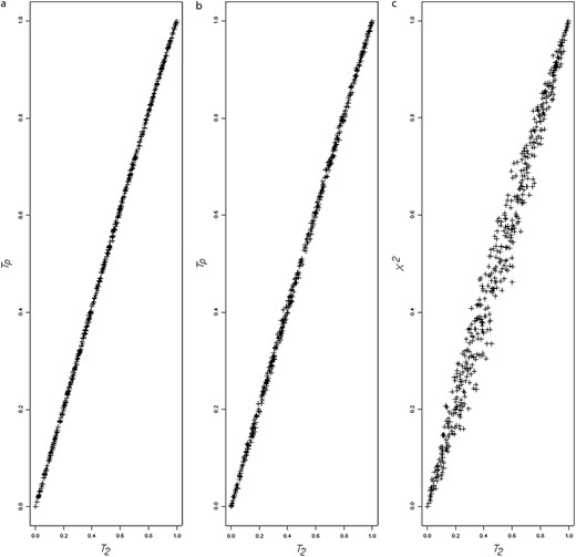
(a) Plots of T2 P-values against the Tp P-values for the known haplotype phase simulations. (b) Plots of T2 P-values against the Tp P-values for the unknown haplotype phase simulations. (c) Plots of T2 P-values against Pearson's χ2 P-values for the known haplotype phase simulations.
Figure 2 shows the correspondence between the two correlation-based test approximations, T1 and T2. Figure 2a illustrates the correspondence for the known haplotype phase case (N = 100; data for Table 1). Figure 2b illustrates a similar correspondence between the P-values for the unknown haplotype phase case (data from simulations to produce “setting I” in Table 8).
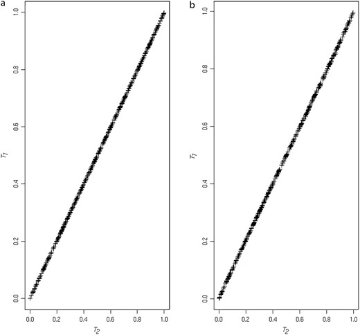
(a) Plots of T2 P-values against T1 P-values for the known haplotype phase simulations. (b) Plots of T2 P-values against T1 P-values for the unknown haplotype phase simulations.
Due to closeness of P-values resulting from the T1 and the T2 tests, and much greater simplicity of the T2-statistic computation, we recommend its usage over the test based on T1.
DISCUSSION
We introduce correlation-based testing for linkage disequilibrium with multiple alleles. Following earlier work by Weir (1979) and Schaid (2004) we adopt the usage of the composite LD that provides robust inference even under conditions of high deviations from HWE. Simulations confirm that the test maintains the proper error rate even when the HWD reaches its maximum value for some of the genotypes. Our approach provides several advantages. The behavior of the proposed method under the hypothesis of no association is found to be consistently closer to the expected than that of other “nonexact” tests included in this study. Values of the statistic SB that we introduced for evaluation of the null distribution of the studied test statistics show that in 35 of 38 experiments, the approximation T2 was closer to its null expected value than the chi-square statistic (Tables 1–9). Power evaluations suggest that the correlation-based tests provide higher power than other tests under the alternatives where associations are present among multiple pairs of alleles (Tables 4–6). The novelty and advantages of our approach also include tractability of the corresponding test statistic, simplicity, and high speed of computations. The relation of the sum of squared LD correlations to chi-square extends the well-known relation for the two-allele case and thus may have implications for the design of genetic association studies. Good power properties of the test based on a simple statistic
Although the method is motivated by testing the LD, the test provides high power when used to detect heterogeneity among samples in contingency tables. For example, the correlation-based test can be used to compare allele or genotype frequencies (columns) between samples from several populations, represented by rows in a contingency table. In this setting, the power is very similar to the power of common tests such as Pearson's chi-square and Fisher's exact test. Further study may be required to fully investigate properties of this test as a general purpose test for detecting interactions and heterogeneity in contingency tables.
A computer program implementing the methods described here is available at (http://www.niehs.nih.gov/research/atniehs/labs/bb/staff/zaykin/rxc.cfm) or by a request to D.V.Z. The provided implementation computes average correlations with the corresponding P-values on the basis of the T2 statistic, using multilocus genotype data. For those P-values that fall below a user-specified threshold, a Monte Carlo P-value is reported as well. This approach allows rapid computations for large collections of loci. Correlation-based tests for contingency tables are implemented as well.
APPENDIX A
APPENDIX B
Tables of population joint frequencies (pij) to provide a specified amount of association (measured by D′) for the power study.
The 4 × 3 table of joint frequencies with the corresponding level of association
pij\D′ | Sum | |||
|---|---|---|---|---|
| 0.0871\0.5 | 0.1567\0.5 | 0.1134\−0.5 | 0.357 | |
| 0.0133\−0.5 | 0.0240\−0.5 | 0.1697\0.5 | 0.207 | |
| 0.0107\−0.5 | 0.0192\−0.5 | 0.1359\0.5 | 0.166 | |
| 0.0174\−0.5 | 0.0313\−0.5 | 0.2213\0.5 | 0.270 | |
| Sum | 0.128 | 0.231 | 0.640 | |
pij\D′ | Sum | |||
|---|---|---|---|---|
| 0.0871\0.5 | 0.1567\0.5 | 0.1134\−0.5 | 0.357 | |
| 0.0133\−0.5 | 0.0240\−0.5 | 0.1697\0.5 | 0.207 | |
| 0.0107\−0.5 | 0.0192\−0.5 | 0.1359\0.5 | 0.166 | |
| 0.0174\−0.5 | 0.0313\−0.5 | 0.2213\0.5 | 0.270 | |
| Sum | 0.128 | 0.231 | 0.640 | |
Absolute values of D′ for this set of simulations are set to be ±0.5.
The 4 × 3 table of joint frequencies with the corresponding level of association
pij\D′ | Sum | |||
|---|---|---|---|---|
| 0.0844\0.5 | 0.0114\−0.5 | 0.0106\−0.5 | 0.106 | |
| 0.1390\−0.5 | 0.1534\0.5 | 0.1437\0.5 | 0.436 | |
| 0.0803\0.5 | 0.0108\−0.5 | 0.0101\−0.5 | 0.101 | |
| 0.2825\0.5 | 0.0381\−0.5 | 0.0356\−0.5 | 0.356 | |
| Sum | 0.586 | 0.214 | 0.200 | |
pij\D′ | Sum | |||
|---|---|---|---|---|
| 0.0844\0.5 | 0.0114\−0.5 | 0.0106\−0.5 | 0.106 | |
| 0.1390\−0.5 | 0.1534\0.5 | 0.1437\0.5 | 0.436 | |
| 0.0803\0.5 | 0.0108\−0.5 | 0.0101\−0.5 | 0.101 | |
| 0.2825\0.5 | 0.0381\−0.5 | 0.0356\−0.5 | 0.356 | |
| Sum | 0.586 | 0.214 | 0.200 | |
Absolute values of D′ for this set of simulations are set to be ±0.5.
The 5 × 5 table of joint frequencies with the corresponding level of association, pij\D′
pij\D′ | Sum | |||||
|---|---|---|---|---|---|---|
| 0.1183\0.20 | 0.0233\−0.20 | 0.0434\−0.21 | 0.0529\−0.20 | 0.0385\−0.20 | 0.277 | |
| 0.0233\−0.20 | 0.0086\−0.20 | 0.0365\0.20 | 0.0196\−0.20 | 0.0142\−0.20 | 0.102 | |
| 0.0228\−0.20 | 0.0084\−0.20 | 0.0357\0.20 | 0.0192\−0.20 | 0.0139\−0.20 | 0.100 | |
| 0.0399\−0.19 | 0.0147\−0.20 | 0.0275\−0.20 | 0.0335\−0.20 | 0.0592\0.20 | 0.175 | |
| 0.0791\−0.19 | 0.0502\0.20 | 0.0545\−0.20 | 0.1143\0.20 | 0.0483\−0.20 | 0.346 | |
| Sum | 0.284 | 0.105 | 0.198 | 0.239 | 0.174 | |
Absolute values of D′ for this set of simulations are set to be in the range 0.19–0.21.
Footnotes
Communicating editor: A. D. Long
Acknowledgement
Shyamal Peddada and David Umbach provided useful discussion. Noah Rosenberg provided STR genotypes for deriving data sets used in the simulation study. Daniel Schaid and Jason Sinnwell provided a program implementing Schaid's S2 test. This research was supported in part by the Intramural Research Program of the National Institutes of Health (NIH), National Institute of Environmental Health Sciences, and by NIH GM 07591.
References
Boos, D. D., and J. Zhang,
Box, G. E. P.,
Cressie, N., and T. R. C. Read,
Excoffier, L., and M. Slatkin,
Fienberg, S. E.,
Ipsen, J., and N. K. Jerne,
Kalinowski, S. T., and P. W. Hedrick,
Holt, D., A. J. Scott and P. D. Ewings,
Larntz, L.,
Lewontin, R. C.,
Oden, N. L.,
Rosenberg, N. A., J. K. Pritchard, J. L. Weber, H. M. Cann, K. K. Kidd et al.,
Waples, R. S.,
Weir, B. S., and C. C. Cockerham,
Weir, B. S., and C. C. Cockerham,
Zapata, C.,
