


Abstract
The doubled-haploid (DH) barley population (Harrington × TR306) developed by the North American Barley Genome Mapping Project (NABGMP) for QTL mapping consisted of 145 lines and 127 markers covering a total genome length of 1270 cM. These DH lines were evaluated in ∼25 environments for seven quantitative traits: heading, height, kernel weight, lodging, maturity, test weight, and yield. We applied an empirical Bayes method that simultaneously estimates 127 main effects for all markers and 127(127−1)/2=8001 interaction effects for all marker pairs in a single model. We found that the largest main-effect QTL (single marker) and the largest epistatic effect (single pair of markers) explained ∼18 and 2.6% of the phenotypic variance, respectively. On average, the sum of all significant main effects and the sum of all significant epistatic effects contributed 35 and 6% of the total phenotypic variance, respectively. Epistasis seems to be negligible for all the seven traits. We also found that whether two loci interact does not depend on whether or not the loci have individual main effects. This invalidates the common practice of epistatic analysis in which epistatic effects are estimated only for pairs of loci of which both have main effects.
EPISTATIC effects are statistically defined as interactions between effects of alleles from two or more genetic loci (Fisher 1918). Interactions, however, are simply deviations from additivity in a general linear model; as such they are often treated as statistical errors. Cockerham (1954) showed that epistatic effects can be partitioned into various epistatic components, e.g.,
Epistasis is an important source of variation contributing to speciation (Wright 1931) because breakdown of a certain combination of alleles already adapted to a local environment will decrease the fitness of the recombinants. However, the importance of epistasis in quantitative traits among less diversified populations is less clear. Some studies showed that the epistatic variance can account for a large proportion of the genetic variance of quantitative traits among progeny of line crosses (Carlborget al. 2005; Malmberg and Mauricio 2005; Malmberget al. 2005). However, the reported epistatic effects of QTL are most likely biased because many studies that did not show any significant epistatic effects are perhaps not reported in the literature, a phenomenon called the Beavis effect (Beavis 1994; Xu 2003b). The censorship of small or null epistatic effects biases the reported results upward. Although efficient methods have been developed for mapping QTL with main effects (Lander and Botstein 1989; Sillanpaa and Arjas 1998; Xu 2003a; Yiet al. 2003a; Wanget al. 2005; Zhanget al. 2005), methods for mapping QTL with epistatic effects are still premature. These methods either utilize models including a single epistatic effect at a time (Holland 1998; Malmberget al. 2005) or apply a model selection strategy that searches for multiple epistatic effects (Carlborget al. 2000; Yiet al. 2003b, 2005). These methods may not guarantee that all important epistatic effects are detected. Recently, Xu (2007) developed an empirical Bayes method that can simultaneously estimate main effects of all individual markers and epistatic effects of all pairs of markers. The algorithm is computationally efficient so that large sets of data can be analyzed within very short computing time.
A doubled-haploid barley population was developed by the North American Barley Genome Mapping Project (Tinkeret al. 1996). Each genotype was replicated ∼25 times. QTL were mapped for seven agronomic traits. On average, there were three to six QTL contributing to the genetic variance of each trait. The results were quite reliable due to the relatively dense marker map, the reasonable sample size, and, more importantly, the large number of replications. Because of this, the data set has been analyzed many times by various investigators to test new statistical models (Xu 2003a; Yiet al. 2003a,b; Zhanget al. 2005; Xu 2007). However, epistatic effects have not been tested in this barley population for all the traits recorded in the experiment. Xu (2007) analyzed only the trait kernel weight (KWT) to demonstrate the application of the empirical Bayes method. No general conclusion was made in that study. We conducted a genomewide analysis of epistatic effects for all the traits using the new method (Xu 2007). The genomewide analysis employed was a true multiple-effect analysis that required no variable selection. All markers and marker pairs were included in a single model and their effects were estimated simultaneously. Since the genome coverage of the markers was quite high, no QTL or QTL pairs would be missed. The results are reliable so that conclusions can be made inclusively about the relative importance of epistasis in the genetic variance of quantitative traits.
MATERIALS AND METHODS
Experimental population:
Data were retrieved from the North American Barley Genome Mapping Project (NABGMP) website (http://gnome.agrenv.mcgill.ca/). The experimental design and results were reported by Tinkeret al. (1996). For the article to be self-contained, the experiment is briefly described here. The population consisted of 145 doubled-haploid (DH) lines of a cross between two related Canadian two-row barley lines, Harrington and TR306. The cross was made by the NABGMP to (1) construct a molecular marker map and (2) locate QTL that affect traits of economic importance. These DH lines were evaluated in 25 replications (environments) for seven quantitative traits: heading (HED), height (HGT), KWT, lodging (LDG), maturity (MAT), test weight (TWT), and yield (YLD). The number of replicates for an individual trait varied from 15 to 29 with an average of 25. The map consisted of 127 markers (mostly RFLPs) distributed over seven chromosomes with an average marker interval of 10.5 cM. The genome coverage of the markers was 1270 cM in length. Tinkeret al. (1996) identified, on average, three to six QTL per trait, collectively explaining 35–50% of the genetic variance. None of the traits were controlled by a major QTL. Some QTL had interaction effects with the environments, but many showed effects that were consistent across environments. Epistatic effects were not investigated in the original study.
The purpose of this analysis was to conduct a genomewide investigation on the epistatic effects for the seven traits. For simplicity, we took the average phenotypic value of each line across the environments as the input phenotype for that line. Because of the large number of replicates, the average phenotypic value of each line approximately represents the genotypic value of that line. All QTL detected would represent those showing consistent effects across environments. The genotype of each marker was coded as
Statistical analysis:
Missing marker genotypes were imputed using information from the nearest nonmissing flanking markers. We first used the genotypes of flanking markers to calculate the conditional probability of the missing marker genotype. We then sampled the genotype of the missing marker from this conditional probability. This is called marker imputation. The missing markers were imputed one at a time from one end of the chromosome to the other end. If two or more consecutive markers were missing, the imputed marker genotype for the first missing marker, combined with the first nonmissing marker in the other side of the second missing marker, was used to calculate the probability of the second missing marker genotype. For example, consider five markers in the order of ABCDE and markers BCD have missing genotypes. The genotype of marker B is generated using information from markers A and E. The genotype of marker C is generated from the imputed genotype of marker B and the genotype of marker E. The genotype of marker D is generated from the imputed genotype of marker C and the genotype of marker E. Once all missing markers were imputed for all individuals, we had a set of imputed marker genotypes for the population. This data set was used as an input data set to conduct the epistatic analysis. We generated 20 imputed samples of the marker genotype data and thus analyzed the data 20 times, one from each imputed marker data set. The estimated parameters represented the average estimates of the 20 imputed samples. The marker distribution was quite even across the genome and thus, for simplicity, we treated each marker as a putative QTL; i.e., we estimated only the effects of markers. If a QTL was located between two markers, its effect would be picked up by the two flanking markers. Hereafter, we use markers and putative QTL interchangeably.
Comparing model (2) to model (1), we can see that
Since the number of model effects is
We used the two-step approach of Xu (2007) to estimate the QTL effects. The first step was a typical random model variance-component analysis. The maximum-likelihood method (Hartley and Rao 1967) was used to estimate the population mean and all the variance components. The number of variance components was 8128, requiring a special algorithm to handle a model with such a large number of parameters (Xu 2007). The second step involved best linear unbiased prediction (BLUP) estimation of the QTL effects given the estimated variance components (Robinson 1991).
The estimated variance components were used only to shrink the estimation of the QTL effects. Because each QTL had its own estimated variance (
How large of an estimated effect is sufficiently large to be declared as “significant”? One can convert each estimated effect into a t-test statistic,
RESULTS
The data were analyzed using a SAS IML program written by Xu (2007). The computer program can be downloaded from our website (http://www.statgen.ucr.edu). The program took ∼2 min to converge for each trait on a Pentium PC with a 3.60-GHz processor and 3.00 GB RAM. The numbers of replications, the estimated means
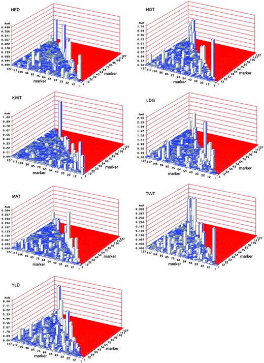
QTL effects for seven agronomic traits of the Harrington × TR306 (H × T) double-haploid barley population. The main (additive) effects are on the diagonals and the epistatic effects are on the left triangle of the 3D plots. Blue prisms represent positive effects (T allele > H allele) and gray prisms represent negative effects (H allele > T allele).
Summary statistics for seven agronomic traits in the Harrington × TR306 double-haploid barley population
Trait | ||||||||
|---|---|---|---|---|---|---|---|---|
| HED | HGT | KWT | LDG | MAT | TWT | YLD | Average | |
| Replication | 29 | 27 | 25 | 17 | 15 | 28 | 28 | 24.12 |
| Mean | 58.97 | 89.18 | 42.50 | 40.43 | 93.53 | 63.24 | 476.11 | |
| Variance | 1.0966 | 8.2071 | 4.9468 | 46.1432 | 0.5403 | 1.1964 | 500.69 | |
| Critical value | 0.0699 | 0.1873 | 0.1512 | 0.4685 | 0.0480 | 0.0684 | 1.4652 | |
| NA | 13 | 9 | 12 | 8 | 14 | 17 | 9 | 11.71 |
| NAA | 5 | 6 | 1 | 11 | 7 | 4 | 9 | 6.14 |
| N | 18 | 15 | 13 | 19 | 21 | 21 | 18 | 17.85 |
| VA | 0.4624 | 2.9319 | 2.2806 | 12.8661 | 0.1868 | 0.3712 | 136.12 | |
| VAA | 0.0505 | 0.4975 | 0.0445 | 5.3988 | 0.0304 | 0.0467 | 52.6325 | |
| VG | 0.5129 | 3.4294 | 2.3251 | 18.2649 | 0.2172 | 0.4179 | 188.7523 | |
| HA | 0.4216 | 0.3572 | 0.4610 | 0.2788 | 0.3458 | 0.3102 | 0.2719 | 0.3495 |
| HAA | 0.0461 | 0.0606 | 0.0089 | 0.1170 | 0.0562 | 0.0390 | 0.1051 | 0.0618 |
| HG | 0.4677 | 0.4178 | 0.4700 | 0.3958 | 0.4020 | 0.3493 | 0.3769 | 0.4114 |
| NA/NAA (0) | 0.8000 | 0.8333 | 1.000 | 0.8181 | 0.8571 | 1.0000 | 1.0000 | 0.9012 |
| NA/NAA (1) | 0.2000 | 0.1667 | 0.0000 | 0.1818 | 0.1428 | 0.0000 | 0.0000 | 0.0987 |
| NA/NAA (2) | 0.0000 | 0.0000 | 0.0000 | 0.0000 | 0.0000 | 0.0000 | 0.0000 | 0.000 |
| HA(MAX) | 0.0968 | 0.1351 | 0.1819 | 0.0993 | 0.1391 | 0.0540 | 0.1032 | 0.1156 |
| HAA(MAX) | 0.0070 | 0.0193 | 0.0089 | 0.0259 | 0.0115 | 0.0109 | 0.0160 | 0.0142 |
NA, number of additive (main) effects; NAA, number of epistatic effects; N, total number of effects; VA, variance of additive effects; VAA, variance of epistatic effects; VG, total genetic variance; HA, proportion of additive variance; HAA, proportion of epistatic variance; HG, proportion of total genetic variance; NA/NAA (0), proportion of epistatic effects between a pair of loci of which both lack main effects; NA/NAA (1), proportion of epistatic effects between a pair of loci of which only one has a main effect; NA/NAA (2), proportion of epistatic effects between a pair of loci of which both have main effects. HA(MAX), HA of the largest additive effect; HAA(MAX), HAA of the largest epistatic effect.
Among the detected epistatic effects, we investigated the proportion of the epistatic effects between pairs of loci that both lack main effects [
DISCUSSION
The epistatic effect model used to analyze the barley data is an oversaturated model. The usual solution to the
The method we employed here is a Bayesian method in terms of estimation of the QTL effects. However, the variance components (
Given the fact that the empirical Bayes method is also a Bayes method, why is it more robust to small sample sizes than the MCMC-based full Bayes methods? Several special properties of the empirical Bayes method may contribute to the robustness. First, the empirical Bayes method does not use a hierarchical model, and thus it infers a smaller number of parameters than the full Bayes methods. Although the empirical Bayes still estimates the variance components, these variance components are estimated separately using a marginal maximum-likelihood (ML) method before the Bayes analysis. By “marginal ML” we mean that the likelihood function is only a function of the variance components and the regression coefficients have been integrated out. The estimates of the variance components do not depend on the regression coefficients. This is clearly in contrast to the full Bayes methods in which the regression coefficients and the variance components are inferred sequentially with the estimate of one parameter depending on estimates of all other parameters. Second, the empirical Bayes method does not involve MCMC sampling for inference of the parameter distribution. The MCMC-based full Bayes methods failed not because they generated wrong estimates but because the Markov chains had never converged to the stationary distribution of the parameters and thus never generated meaningful estimates of the parameters. Third, the empirical Bayes method employed in this study infers the marginal posterior mean of each regression coefficient, with other regression coefficients integrated out. Therefore, the estimate of one regression coefficient does not depend on the estimates of other regression coefficients. This clearly has improved the robustness of the method to small sample size.
The justification for the robustness of the empirical Bayes method to small sample sizes does not mean that the empirical Bayes method can deal with a population with an infinitely small sample size. There is a limit below which any method will fail because the data are just too small to contain sufficient information to make any inferences. Is a sample size of 145 DH lines sufficient for QTL mapping? The answer is probably no in general (Beavis 1994; Melchingeret al. 1998), but 145 lines seem to be sufficient to infer large-effect QTL in this particular barley population. One reason is that the phenotypic value of each line in each environment was measured by the average value of several plants, all with the same genotype (Tinkeret al. 1996). The mean phenotypic value (plot mean) of a line in a particular environment already represented approximately the genotypic value of that line in that environment. The variance of plot means across environments was largely due to
Although the empirical Bayes method worked well for this data set, the sample size was not sufficiently large to shrink all small effects to zero. Many spurious QTL effects still occurred. Therefore, we adopted a permutation test to find a suitable criterion to select those QTL with effects sufficiently large to be declared as significant. Theoretically, the critical value should be obtained from many reshuffled samples, say 1000. In this study, the number of effects in the model was so large that 20 reshuffled samples appeared to be sufficient. We found that the variance of the critical values obtained from multiple reshuffled samples was small. For example, the average critical value for HED at
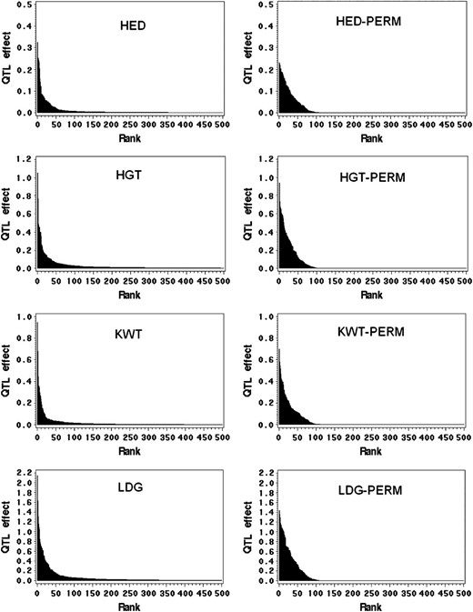
Plots of QTL effects against the rankings (in descending order) for four agronomic traits in the Harrington × TR306 double-haploid barley population. Each plot in the right column represents a randomly reshuffled sample for the corresponding trait in the left column. The total number of effects included in the model was 8128, but the plots reflect the top 500 effects only (truncated data).
Usually, significance tests are not required in Bayesian analysis; only frequentists emphasize significance tests. We employed a permutation test to make inferences about the significance of a QTL effect. This is a hybrid approach between Bayesian and frequentist approaches. The purpose of this study was not for QTL detection; rather it was intended to assess the importance of epistasis relative to additivity for economically important quantitative traits in barley. If QTL detection were the purpose, simply reporting all QTL effects that explain more than
The epistatic effects defined in our model are different from the orthogonal contrasts defined by Cockerham (1954) and recently reiterated by Kao and Zeng (2002) and Zenget al. (2005). Kao and Zeng called Cockerham's epistatic effects the statistical parameters and the epistatic effects defined here the genetic parameters. The genetic parameters were also called physiological parameters by Cheverud and Routman (1995). The orthogonal contrasts can be expressed as linear functions of the genetic effects defined in our model. This means that Cockerham's epistatic effects are functions of the main effects defined in our model. This may justify Kao and Zeng (2002) for estimating epistatic effects only for loci that both have main effects because main effects contribute to the orthogonalized epistatic effects. The presence of epistatic effects between two loci defined in our study does not depend on whether or not the two loci both have main effects. This has been proved by the analysis of this experiment. Take trait HED, for example; we detected five epistatic effects, but none of the effects involved two loci that both had significant main effects. One epistatic effect involved a pair of loci of which only one had a significant main effect (1/5 = 0.2). The remaining four epistatic effects (4/5 = 0.8) involved pairs of loci that both lack main effects. In traditional QTL mapping, people normally scan the genome for QTL with main effects. Once QTL with main effects are identified, an epistatic model is fit to examine the epistatic effects only between the QTL that have main effects. This approach certainly has no logical basis. We would not be able to detect any epistatic effects for the barley data if this approach had been taken.
Our conclusion for the barley data analysis was that epistatic variance does contribute to the genetic variance. However, the cumulative contribution from significant epistatic effects is very small relative to that from the additive effects. This discovery was consistent for all the seven traits investigated. A recent study using F2 progeny of a cross between two inbred mice for obesity-related traits showed that many epistatic effects were significant, but they were all small in magnitude relative to the additive effects (Yiet al. 2006). The largest main-effect QTL contributed ∼20% of the trait variance but the largest epistatic effect accounted for only ∼5% of the trait variance. The result from the mice experiment was similar to that from the barley analysis. Yiet al. (2006) used a Bayesian model selection method to analyze the mice data. Although the model used by Yiet al. (2006) was not saturated, it was a multiple-effects model in which multiple main effects and epistatic effects were simultaneously estimated in a single model, a feature also shared by the method used this study. Therefore, simultaneous estimation of all model effects seemed to support the notion that epistasis is not an important contributor to the genetic variance of less diversified varieties of crops or breeds of animals.
Footnotes
Communicating editor: N. Takahata
Acknowledgement
We are grateful to two anonymous reviewers for their useful comments and suggestions on the first version of this manuscript, which have significantly improved its current presentation. This research was supported by the National Institutes of Health grant R01-GM55321 and the National Science Foundation grant DBI-0345205 to S.X.
References
Beavis, W. D.,
Carlin, B. P., and T. A. Louis,
Fisher, R. A.,
George, E. I., and R. E. Mcmulloch,
George, E. I., and R. E. Mcmulloch,
Holland, J. B.,
Jannink, J.-L.,
Lindley, D. V., and A. F. M. Smith,
Robinson, G. K.,
Tibshirani, R.,
Tinker, N. A., D. E. Mather, B. G. Rossnagel, K. J. Kasha, A. Kleinhofs et al.,
Xu, S.,
