Abstract
An analytic expression of conditional expectation of transient gamete frequency, given that one of the two loci remains polymorphic, is obtained in terms of the diffusion process by calculating the moments of the distribution. Using this expression, a model where linkage disequilibrium is introduced by a single mutation is considered. The conditional expectation of the gamete frequency given that the locus with the mutant allele remains polymorphic is presented. The behavior is significantly different from the monotonic decrease observed in the deterministic model without random genetic drift.
WITH respect to random genetic drift for the one-locus problem, the state of steady decay was first obtained correctly by Wright (1931). However, in this study it was assumed that the state of steady decay had already been attained. By calculating the moments of the distribution, Kimura (1955a) obtained the complete expression of the transient probability density for the unfixed class, which shows how the process leads to the state of steady decay. It was found that after 2N generations the distribution becomes almost flat, where N is the effective population size.
Since each mutant ultimately becomes either fixed or lost, the steady state will be attained only if linear evolutionary pressures, such as mutation, operate. For the two-locus problem, the steady state has been discussed in terms of the diffusion process (Ohta and Kimura 1969b, 1970; Ethier and Nagylaki 1989) and the genealogical process (Griffiths 1981; Hudson 1983, 1985; Golding 1984; Ethier and Griffiths 1990). In contrast, in situations without linear evolutionary pressures, how the process eventually leads to the state of steady decay has not been studied, with the exception of several functions that vanish at the absorbing boundaries (Hill and Robertson 1968; Ohta and Kimura 1969a; Littler 1973). Despite the fact that the two-locus problem is uniquely characterized by gamete frequencies, the transient behavior of them has not been examined.
In this article, I derive an analytic expression of conditional expectation of the transient gamete frequency, given that one of the two loci remains polymorphic, in terms of the diffusion process. This expression shows how it ultimately leads to the asymptotic value. Using this expression, a model where linkage disequilibrium is introduced by a single mutation is discussed.
THE DIFFUSION PROCESS OF THE TWO-LOCUS PROBLEM
Consider a random-mating population with an effective population size of
N. We measure time
T in units of 2
N generations. Let
A1 and
A2 be a pair of alleles with initial allele frequencies that are
p and 1 −
p, respectively, and the allele frequencies at time
T are
X and 1 −
X, respectively.
Kimura (1955a) obtained an analytic expression of the transient probability density for the unfixed class. In what follows lowercase letters of random variables represent their values. Let ϕ(
p,
x;
T) be the probability density. The probability that the locus remains polymorphic was also given,
where
Pm(
z) represents the Legendre polynomial.
Next, we discuss the expectation of the allele frequency. In general, since we cannot observe a polymorphism that has been lost, a polymorphism can be observed only for an unfixed class. Thus, the obvious relation
E[
X] =
p is nonsense from the perspective of observation. We have interest in the conditional expectation of the frequencies given that a polymorphism is retained. By using the expression of the transient fixation probability, which was given by
Kimura (1955a), we obtain the conditional expectation of the allele frequency for the unfixed class,
where
where
I(0,1)(
X) represents the indicator function of the open interval (0, 1) and
f(1;
T) represents the transient fixation probability of the allele
A1. The asymptotic value of the conditional expectation of the allele frequency is
which agrees with the fact that the conditional distribution becomes uniform asymptotically.
Let us assume two loci
A and
B in which pairs of alleles
A1,
A2 and
B1,
B2 are segregating, and let the initial frequencies of gametes
A1B1,
A1B2,
A2B1, and
A2B2 be, respectively,
g1,
g2,
g3, and 1 − (
g1 +
g2 +
g3), and let the frequencies of them at time
T be, respectively,
X1,
X2,
X3, and 1 − (
X1 +
X2 +
X3). Let the initial frequencies of alleles
B1 and
B2 be, respectively,
q and 1 −
q, and let the frequencies of them at time
T be
Y and 1 −
Y, respectively. Let
D =
g1(1 −
g1 −
g2 −
g3) −
g2g3 be the initial value of the linkage disequilibrium coefficient and
Z =
X1(1 −
X1 −
X2 −
X3) −
X2X3 be the value of the linkage disequilibrium coefficient at time
T. We have
Let c be the recombination fraction between the two loci, and we set ρ = 4Nc. We do not discuss where c = 0, since the problem reduces to the multiallelic one-locus problem that has previously been discussed by Kimura (1955b). For the deterministic model without random genetic drift, we have x = p, y = q, and z = De−ct.
The probability density for the gamete frequencies
satisfies the following Kolmogorov backward equation,
(
Ohta and Kimura 1969a), where δ
ij represents Kronecker's delta. Although the probability density itself is unknown,
Ohta and Kimura (1969a) obtained expectations of functions
which were discussed by
Hill and Robertson (1968). The process is defined in a tetrahedron 0 ≤
x1 ≤
x1 +
x2 ≤
x1 +
x2 +
x3 ≤ 1. By changing variables from the gamete frequencies to the variables
x,
y, and
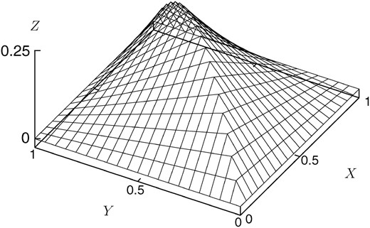
z, the region is transformed into a three-dimensional region, the upper surface of the boundary of which is depicted in
Figure 1. On the peripheral edges, which is the periphery of the square 0 ≤
x ≤ 1, 0 ≤
y ≤ 1, one of the two loci is monomorphic. At the points (1, 1, 0), (1, 0, 0), (0, 1, 0), and (0, 0, 0), one of the gametes
A1B1,
A1B2,
A2B1, and
A2B2 fixes, respectively. We represent the inside of the region as
\(\mathcal{D}\)
. The expectation of the linkage disequilibrium coefficient is
(
Hill and Robertson 1968), and the squared standard linkage deviation tends to
when ρ is large (
Ohta and Kimura 1969a).
Figure 1.—
The upper surface of the boundary of the region in which the diffusion process is defined.
Next, we discuss the expectation of the gamete frequencies. In the same manner as for the functions (4) and the linkage disequilibrium measure, we obtain the expectation of the gamete frequency
X1:
However, in contrast to the functions (4) and the linkage disequilibrium coefficient, the gamete frequencies do not vanish at the peripheral edges. The expectation takes over not only the inside of the region
\(\mathcal{D}\)
, but also the peripheral edges. As obtained by
Ohta (1968),
\(\mathrm{lim}_{T{\rightarrow}{\infty}}E[X_{1}]\)
gives the fixation probability of the gamete
A1B1. Thus, the expectation of the gamete frequency
X1 can be rewritten as
where ϕ
x=1 and ϕ
y=1 represent the probability density for the open intervals
x = 1,
y ∈ (0, 1),
z = 0 and
x ∈ (0, 1),
y = 1,
z = 0, respectively, and
f(1, 0, 0;
T) represents the transient fixation probability of the gamete
A1B1 at time
T. With respect to the one-locus problem, as discussed above, we are interested in the conditional expectation of the gamete frequencies given that polymorphism is retained.
CONDITIONAL EXPECTATION OF GAMETE FREQUENCY
Let us suppose a model whereby linkage disequilibrium is introduced by a single mutation, as considered by
Nei and Li (1980) regarding the association between electromorphs and inversion chromosomes in Drosophila. We assume that locus
A has remained monomorphic with the wild-type allele
A2 and that locus
B, in which a pair of alleles
B1 and
B2 (electromorphs) are segregating, has allele frequencies
q and 1 −
q, respectively. Then, the mutation introduces the mutant allele (inversion chromosome)
A1 to locus
A of one of the allele
B1 bearing chromosomes. This model specifies the initial allele frequency of
A1 as
p = 1/2
N, the initial gamete frequencies as
g1 =
p,
g2 = 0, and
g3 =
q −
p, and the initial value of the linkage disequilibrium measure as
D =
p(1 −
q); however, the following expressions hold regardless of these relations. In this model, a polymorphism at locus
A is important since allele
A1 is prone to be lost by random genetic drift. In addition, locus
B may be regarded as a marker polymorphism to detect the mutant. In this article, we consider the conditional expectation given that locus
A remains polymorphic. It might seem that this condition is similar to that described by
Kaplan and Weir (1992). They discussed conditional expectation of the linkage disequilibrium measure, which was defined by
Nei and Li (1980), given that a polymorphism is observed at locus
B. They assumed that the allele frequency of
A1 is constant and that locus
B follows the infinite-allele model assumption. Moreover, they considered the steady state. Thus, their model differs from that described here, and the condition that locus
A remains polymorphic is meaningful for our diffusion process, which ultimately leads to monomorphism. Note that this condition nearly equates to a condition that both of the two loci remain polymorphic for large-size populations, since the probability that a polymorphism at locus
A is lost earlier than that at locus
B is given by
Karlin and McGregor (1968),
which is almost unity unless the allele frequency
q is very small.
By expression (5), we have
The expressions for the other gamete frequencies
X2 and
X3 can be obtained in the same manner. To calculate the limit of the expectation
\(\mathrm{lim}_{n{\rightarrow}{\infty}}E[X^{n}Y]\)
, we consider some moments. For convenience, we denote
Making use of the Kolmogorov backward
equation (3), the moments μ
ℓ,m,n satisfy a differential equation:
It is worthwhile to note that
E[
XℓYmX1n] satisfies a recurrence relation on the two-locus sampling distribution by
Golding (1984;
Ethier and Griffiths 1990).
The moments μ
n,0,1 satisfy a differential equation,
and the differential equation has the solution of the form
where
with the initial condition
In
appendix a it is shown that
where
\(T_{m}^{1}(z)\)
represents the Gegenbauer polynomial, which is also represented as
\(C_{m}^{3/2}(z)\)
.
The moments μ
n,1,0 satisfy a differential equation,
and the differential equation has the solution of the form
where
with the initial condition
The recurrence relation (9) can be expressed by a matrix equation,
\(\mathbf{\mathrm{Af}}{=}\mathbf{\mathrm{c}}\)
with vectors
\(\mathbf{\mathrm{f}}_{k}{=}F_{k}^{(m)},{\,}\mathbf{\mathrm{c}}_{k}{=}2kC_{k{-}1}^{(m)},(k{=}m,{\,}m{+}1,{\ldots},{\,}n)\)
. The determinant of the matrix
A is
which has zeros at ρ = 2 + 2ℓ, (ℓ = 1, 2, 3, …). These zeros are due to degeneracy of the eigenvalues. Since we are not interested in the specific points of ρ, we discuss the case that the inverse matrix exists in the following, although the calculation is straightforward for each point ρ = 2 + 2ℓ, (ℓ = 1, 2, 3, …). By applying the inverse matrix, we obtain
It is shown in
appendix b that the finite series inside of the brackets follows an identity:
Thus, we obtain
By using (12) and the orthogonal property of the Gegenbauer polynomial,
we obtain the general expression for
\(E^{(m)}_{n}\)
from (10),
We observe the limit,
which agrees with the limit theorem given by
Ethier (1979).
We observe the limits of
\(F^{(m)}_{n}\)
and
\(E^{(m)}_{n}\)
,
and
respectively.
By using these results for the moments, we arrive at the analytic expression of (6):
We observe the limit,
which shows the deterministic behavior of the gamete frequency
X1 without random genetic drift, as expected.
We observe the asymptotic form,
The conditional expectation of the gamete frequency
X1 given that locus
A remains polymorphic is
where the denominator is given by (1). The asymptotic value of the conditional expectation of the gamete frequency
X1 is
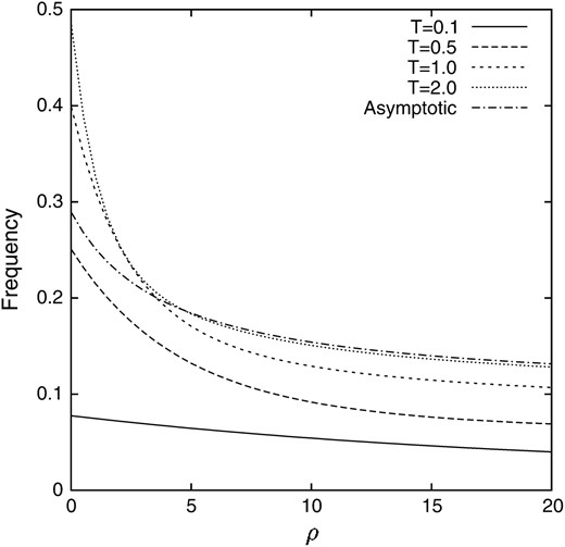
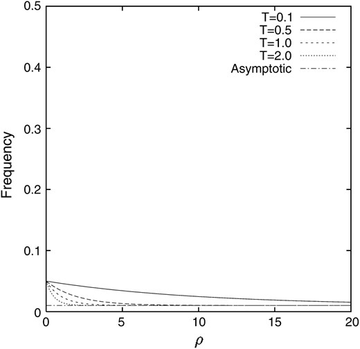
In contrast to the deterministic model without random genetic drift, the value is higher than pq, to which the deterministic model tends, and depends on ρ. Note that the second term of the asymptotic value in (14) represents the conditional covariance between the frequencies of the alleles A1 and B1. The process of the change in the conditional expectation of the gamete frequency X1 when the linkage disequilibrium is introduced into a population as p = 1/2N = 0.05 and q = 0.2 is illustrated in Figure 2. It can be seen that after 4N generations (T = 2.0) the conditional expectation of the gamete frequency X1 almost reaches the asymptotic value for large ρ, although 4N generations is still not enough for small ρ. It can also be seen that the conditional expectation of the gamete frequency X1 does not show monotonic behavior for small ρ. It increases rapidly and then decreases to the asymptotic value. For comparison, the counterpart in the deterministic model is also illustrated in Figure 3
Figure 2.—
The conditional expectation of the gamete frequency X1 given that locus A keeps polymorphism. p = 0.05 and q = 0.2.
Figure 3.—
The gamete frequency X1 in the deterministic model without random genetic drift. p = 0.05 and q = 0.2.
.
To observe the frequency of the allele
B1 within the allele
A1 bearing chromosomes, let us consider a ratio of the conditional expectation of the gamete frequency
X1 to that of the allele frequency
X,
where the denominator is given by (2). The asymptotic value is
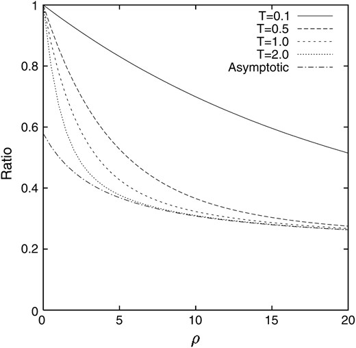
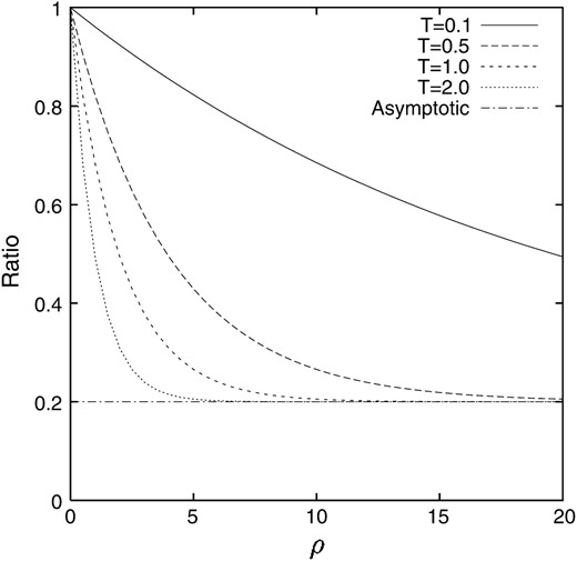
In contrast to the deterministic model without random genetic drift, the value is higher than q, to which the deterministic model tends, and depends on ρ. The process of the change in the ratio of the conditional expectation of the gamete frequency X1 to that of the allele frequency X when the linkage disequilibrium is introduced into a population as p = 1/2N = 0.05 and q = 0.2 is illustrated in Figure 4. It can be seen that after 4N generations (T = 2.0) the ratio almost reaches the asymptotic value for large ρ, although 4N generations is still not enough for small ρ. For comparison, the counterpart in the deterministic model is also illustrated in Figure 5. It can be seen that the discrepancy between our model and the deterministic model is significant for small ρ.
Figure 4.—
The ratio of the conditional expectation of the gamete frequency X1 given that locus A keeps polymorphism to that of the allele frequency X. p = 0.05 and q = 0.2.
Figure 5.—
The ratio of the gamete frequency X1 to the allele frequency X in the deterministic model without random genetic drift. p = 0.05 and q = 0.2.
DISCUSSION
The analytic expression of conditional expectation of transient gamete frequency given that one of the two loci remains polymorphic was obtained in terms of the diffusion process by calculating the moments of the distribution. This expression is general and independent from models that introduce linkage disequilibrium into a population.
We considered the model that linkage disequilibrium is introduced by a single mutation and association between the mutant allele A1 and the allele B1, which filled the other locus of the chromosome on which the mutation occurred. Because the allele A1 is prone to be lost by random genetic drift, the conditional expectation of the frequency of the gamete A1B1 given that locus A remains polymorphic is meaningful. The behavior is significantly different from the monotonic decrease in the deterministic model without random genetic drift. After 4N generations, the conditional expectation of the gamete frequency almost reaches the asymptotic value for large ρ, although 4N generations is still not enough for small ρ. The asymptotic value is larger than the product of the initial allele frequencies to which the deterministic model tends and depends on the recombination fraction between the two loci. Note that the conditional expectation of the linkage disequilibrium coefficient vanishes asymptotically in a similar manner to that in the deterministic model. This observation demonstrates the obvious fact that the linkage disequilibrium measure is not enough to characterize the two-locus problem uniquely.
APPENDIX A
Since the Gegenbauer polynomial is orthogonal on the interval [−1, 1], the right-hand terms of (7) can be represented in terms of the Gegenbauer polynomials of which degrees are up to
n − 1 as
where we set
z = 1 − 2
p. Multiplying
\((1{-}z^{2})T_{m{-}1}^{1}(z)\)
on both sides of the equation and using the orthogonal property (13), we have
An integral transform of (1 −
z)(1 +
z)
n by the Gegenbauer polynomial is
(
Erdélyi 1954). Thus, we have
APPENDIX B
It is straightforward to check the identity (11) for
m =
n. For 1 ≤
m ≤
n − 1, the finite series can be expressed by the truncated hypergeometric series,
where
yn(
a,
b,
c,
z) is the truncated hypergeometric series. The truncated hypergeometric series can be expressed in terms of the generalized hypergeometric series,
(
Erdélyi 1953), where
is the generalized hypergeometric series. Thus, we have an identity for the truncated hypergeometric series:
By using the identity for the truncated hypergeometric series, we obtain
Acknowledgement
I acknowledge the continuous encouragement offered by T. Gojobori. Also, I thank M. Notohara, A. Simizu, and two anonymous reviewers for comments on an earlier version of this manuscript.
References
Erdélyi, A. (Editor),
1953
Higher Transcendental Functions, Vol. I. McGraw-Hill, New York.
Erdélyi, A. (Editor),
1954
Tables of Integral Transforms, Vol. II. McGraw-Hill, New York.
Ethier, S. N.,
1979
A limit theorem for two-locus diffusion models in population genetics.
J. Appl. Probab.
16
: 402
–408.
Ethier, S. N., and R. C. Griffiths,
1990
On the two-locus sampling distribution.
J. Math. Biol.
29
: 131
–159.
Ethier, S. N., and T. Nagylaki,
1989
Diffusion approximation of the two-locus Wright-Fisher model.
J. Math. Biol.
27
: 17
–28.
Golding, G. B.,
1984
The sampling distribution of linkage disequilibrium.
Genetics
108
: 257
–274.
Griffiths, R. C.,
1981
Neutral two-locus multiple allele model with recombination.
Theor. Popul. Biol.
19
: 169
–186.
Hill, W. G., and A. Robertson,
1968
Linkage disequilibrium in finite populations.
Theor. Appl. Genet.
38
: 226
–231.
Hudson, R. R.,
1983
Property of a neutral allele model with intragenic recombination.
Theor. Popul. Biol.
23
: 183
–201.
Hudson, R. R.,
1985
The sampling distribution of linkage disequilibrium under an infinite allele model without selection.
Genetics
109
: 611
–631.
Littler, R. A.,
1973
Linkage disequilibrium in two-locus, finite, random mating models without selection or mutation.
Theor. Popul. Biol.
4
: 259
–275.
Kaplan, N. L., and B. S. Weir,
1992
Expected behavior of conditional linkage disequilibrium.
Am. J. Hum. Genet.
51
: 333
–343.
Karlin, S., and J. McGregor,
1968
Rates and probabilities of fixation for two locus random mating finite population without selection.
Genetics
58
: 141
–159.
Kimura, M.,
1955
a Solution of a process of random genetic drift with a continuous model.
Proc. Natl. Acad. Sci. USA
41
: 144
–150.
Kimura, M.,
1955
b Random genetic drift in multi-allelic locus.
Evolution
9
: 419
–435.
Nei, M., and W-H. Li,
1980
Non-random association between electromorphs and inversion chromosomes in finite populations.
Genet. Res.
35
: 65
–83.
Ohta, T.,
1968
Effect of initial linkage disequilibrium and epistasis on fixation probability in a small population, with two segregating loci.
Theor. Appl. Genet.
38
: 243
–248.
Ohta, T., and M. Kimura,
1969
a Linkage disequilibrium due to random genetic drift.
Genet. Res.
13
: 47
–55.
Ohta, T., and M. Kimura,
1969
b Linkage disequilibrium at steady state determined by random genetic drift and recurrent mutation.
Genetics
63
: 229
–238.
Ohta, T., and M. Kimura,
1970
Linkage disequilibrium between two segregating nucleotide sites under the steady flux of mutations in a finite population.
Genetics
68
: 571
–580.
Wright, S.,
1931
Evolution in Mendelian populations.
Genetics
16
: 97
–159.
© Genetics 2005


