


Abstract
We present a maximum-likelihood-ratio test of the standard neutral model, using multilocus data on polymorphism within species and divergence between species. The model is based on the Hudson-Kreitman-Aguadé (HKA) test, but allows for an explicit test of selection at individual loci in a multilocus framework. We use coalescent simulations to show that the likelihood-ratio test statistic is conservative, particularly when the assumption of no recombination is violated. Application of the method to polymorphism data from 18 loci from a population of Arabidopsis lyrata provides significant evidence for a balanced polymorphism at a candidate locus thought to be linked to the centromere. The method is also applied to polymorphism data in maize, providing support for the hypothesis of directional selection on genes in the starch pathway.
THE neutral theory of molecular evolution predicts that the amount of within-species diversity should be correlated with levels of between-species divergence, due to the dependence of both on the neutral mutation rate (Kimura 1983). The widely used HKA test (Hudson et al. 1987) evaluates the fit of polymorphism and divergence data to this prediction, as a test for natural selection against the null hypothesis of neutrality. The method involves the use of within-species polymorphism data on a sample from one species and sequence divergence from a related species, so that the relative amounts of polymorphism and divergence can be compared across loci. When applied to multilocus data, the HKA test assesses the overall fit of the data to a neutral model that assumes the same ratios of polymorphism and divergence at each locus. The marginal contributions of each locus to the multilocus chi-square statistic, or the results of multiple pairwise HKA tests, are often used to assess which loci contribute most to any observed departure from neutrality (e.g., Moore and Purugganan 2003). This approach, however, does not provide a way of rigorously comparing different models, for example, to test for selection at a specific locus.
The full neutral model thus has r + 1 parameters: a θ parameter for each locus, plus the shared divergence time parameter. The maximum log-likelihood under this model can thus be compared with the maximum log-likelihood with a common u parameter for all loci (u1 = u2 = … = ur) to provide a likelihood-ratio test for the null hypothesis of a common mutation rate for all loci.
In this model, k measures the degree to which diversity is increased or decreased by the action of selection at locus r. The fit under this model can then be compared to that under the alternative of no selection at the rth locus by a likelihood-ratio test.
For changes with lower likelihood, the probability of acceptance is determined by multiplying the difference in log-likelihood by a factor f of 50. After 10,000 iterations, this acceptance probability is reduced to a factor f of 0.5 times the difference in log-likelihoods for 1000 iterations and then returned to the original value. The Markov chain is run multiple times, using different starting parameters and different random-number seeds to ensure convergence. To test a difference between two models that yield maximum likelihoods L1 and L2, we use the likelihood-ratio test statistic 2(ln L2 − ln L1), i.e., twice the difference in log-likelihoods between two models. A program written in C++ to carry out the method is available for download at www.yorku.ca/stephenw.
Here we consider four likelihood models:
- Model 1 (1 free parameter): fixed mutation (u1 = u2 = … ur), no selectionModel 2 (r free parameters, where r = number of loci): free mutation (all θi estimated independently), no selection (k1 = k2 = … kr = 1)\[\left(k_{1}\ =\ k_{2}\ =\ {\ldots}\ k_{r}\ =\ 1\right)\]
Model 3 (1 free parameter): fixed mutation (u1 = u2 = … ur), selection at candidate locus l (kl estimated, k2 = k3 = … ki≠l = 1)
Model 4 (r + 1 free parameters): free mutation (all ui estimated independently), selection at candidate locus l (kl estimated, k1 = k2 = … ki≠l = 1).
We have applied the method to polymorphism data for 18 genes (supplementary Table 1
Maximum-likelihood analysis of synonymous polymorphism and divergence for A. lyrata
Model | Description | ka | ln L | Model comparison | Likelihood-ratio statistic (d.f.) | Pb |
|---|---|---|---|---|---|---|
| 1 | Fixed mutation, no selection | — | −131.8 | — | ||
| 2 | Free mutation, no selection | — | −95.9 | M2 vs. M1 | 71.8 (17) | 8.4 × 10⁻⁹ |
| 3 | Fixed mutation, selection | 9.1 | −119.8 | M3 vs. M1 | 24 (1) | 9.6 × 10⁻⁷ |
| 4 | Free mutation, selection | 4.3 | −91.4 | M4 vs. M3 | 56.8 (17) | 3.5 × 10⁻⁶ |
| M4 vs. M2 | 9 (1) | 2.7 × 10⁻³ |
Selection parameter for the gene AT1G36310.
Probability of likelihood-ratio test, assuming the χ2 distribution.
at http://www.genetics.org/supplemental/) from a single Icelandic population of Arabidopsis lyrata, using divergence estimates from A. thaliana (S. Wright and D. Charlesworth, unpublished data). These loci have an average of 126 synonymous sites and 3.9 segregating synonymous sites, and the sample size averaged 16.7 haploid genomes. For this data set, 100,000 chains were found to be sufficient for convergence, which took ∼5 min to run on a 2.8-GHz Pentium computer. To evaluate the behavior of the model, and to assess the fit of the likelihood ratio statistic to the χ2 approximation, we ran neutral coalescent simulations (Hudson 2002) for 18 loci, with divergence time, sample size, and θ parameter values chosen to match estimates from the A. lyrata data set. All coalescent simulations included a population split and a single sample from the outgroup species, so that polymorphism and divergence were both estimated from the same coalescent process. We ran two sets of 1000 simulations; the first had no intragenic recombination, and the second included intragenic recombination, with values of the population recombination parameter ρ = 4Ner estimated for each locus using genetic mapping data from A. thaliana, as previously described (Wright et al. 2003). Across loci, the assumed per-locus values of ρ ranged from 0.3 to 60, and the ratio ρ/θ ranged from 0.02 to 10. Our candidate locus for selection (“locus 10”) is a gene thought to be linked to the centromere, AT1G36310, which had been hypothesized (S. Wright and D. Charlesworth, unpublished data) to be linked to a site under selection, due to increased hitchhiking in a region of reduced recombination.
To test the assumption of heterogeneity in mutation rates with this data set, we compare a fixed-rate model (model 1) with a free-rate model (model 2). Significance is assessed using a likelihood-ratio test, using χ2 with r − 1 = 17 d.f. Model 2 provides a highly significant improvement to the likelihood compared with model 1, indicating the existence of heterogeneity in mutation rates across loci (Table 1). This highlights the importance of incorporating mutation rate variation into parameter estimation (e.g., Wall 2003) and tests of natural selection. Simulations show that likelihood estimation of divergence and mutation parameters perform well under the neutral model, even in the presence of intragenic recombination (Table 2)
Results of simulations of parameter estimates using the maximum-likelihood estimators based on polymorphism and divergence
No intragenic recombination | Intragenic recombination | ||||||
|---|---|---|---|---|---|---|---|
| Parameter | Valuea | Mean | Median | Standard error | Mean | Median | Standard error |
| T | 17.83 | 18.50 | 18.18 | 0.0982 | 18.22 | 18.04 | 0.0840 |
| θ1 | 0.0084 | 0.0084 | 0.0082 | 7.4 × 10⁻⁵ | 0.0083 | 0.0081 | 6.6 × 10⁻⁵ |
| θ2 | 0.0070 | 0.0068 | 0.0066 | 6.4 × 10⁻⁵ | 0.0069 | 0.0069 | 6.0 × 10⁻⁵ |
| θ3 | 0.0067 | 0.0066 | 0.0066 | 6.5 × 10⁻⁵ | 0.0066 | 0.0065 | 6.1 × 10⁻⁵ |
| θ4 | 0.0066 | 0.0066 | 0.0064 | 6.2 × 10⁻⁵ | 0.0066 | 0.0065 | 5.7 × 10⁻⁵ |
| θ5 | 0.0049 | 0.0049 | 0.0048 | 4.9 × 10⁻⁵ | 0.0049 | 0.0049 | 4.7 × 10⁻⁵ |
| θ6 | 0.0085 | 0.0085 | 0.0084 | 7.0 × 10⁻⁵ | 0.0085 | 0.0083 | 6.5 × 10⁻⁵ |
| θ7 | 0.0052 | 0.0052 | 0.0050 | 5.4 × 10⁻⁵ | 0.0052 | 0.0050 | 5.0 × 10⁻⁵ |
| θ8 | 0.0068 | 0.0068 | 0.0067 | 6.0 × 10⁻⁵ | 0.0069 | 0.0068 | 5.2 × 10⁻⁵ |
| θ9 | 0.0090 | 0.0089 | 0.0087 | 7.5 × 10⁻⁵ | 0.0090 | 0.0087 | 7.0 × 10⁻⁵ |
| θ10 | 0.0282 | 0.0280 | 0.0275 | 1.7 × 10⁻⁴ | 0.0284 | 0.0278 | 1.6 × 10⁻⁴ |
| θ11 | 0.0105 | 0.0103 | 0.0101 | 8.1 × 10⁻⁵ | 0.0106 | 0.0104 | 8.1 × 10⁻⁵ |
| θ12 | 0.0127 | 0.0126 | 0.0124 | 9.2 × 10⁻⁵ | 0.0129 | 0.0127 | 9.3 × 10⁻⁵ |
| θ13 | 0.0079 | 0.0078 | 0.0075 | 6.4 × 10⁻⁵ | 0.0079 | 0.0078 | 6.2 × 10⁻⁵ |
| θ14 | 0.0077 | 0.0076 | 0.0073 | 6.7 × 10⁻⁵ | 0.0076 | 0.0076 | 6.3 × 10⁻⁵ |
| θ15 | 0.0131 | 0.0131 | 0.0129 | 9.1 × 10⁻⁵ | 0.0131 | 0.0130 | 9.0 × 10⁻⁵ |
| θ16 | 0.0115 | 0.0113 | 0.0112 | 8.8 × 10⁻⁵ | 0.0115 | 0.0114 | 8.0 × 10⁻⁵ |
| θ17 | 0.0087 | 0.0086 | 0.0083 | 7.8 × 10⁻⁵ | 0.0087 | 0.0085 | 7.4 × 10⁻⁵ |
| θ18 | 0.0054 | 0.0054 | 0.0052 | 5.2 × 10⁻⁵ | 0.0054 | 0.0053 | 5.1 × 10⁻⁵ |
Values of divergence time and population mutation parameters used in simulations.
.
To test for selection, we first use the standard multilocus HKA test for comparison, using the program of J. Hey (http://lifesci.rutgers.edu/heylab/DistributedProgramsandData.htm#HKA). The standard multilocus HKA test for these 18 loci shows a significant departure from neutral expectation (χ2 = 43.6, P < 0.001), suggesting the action of natural selection at some loci. However, no individual locus shows evidence for selection using the HKA test; the maximum marginal χ2 deviation is contributed by the polymorphism cell for the candidate locus (locus 10), which shows elevated levels of polymorphism, but this value is not significantly greater than expected under neutral coalescent simulations (P = 0.13). Furthermore, pairwise HKA tests comparing locus 10 to all other loci give 7 of 17 significant tests at the 5% level. While the above results are suggestive of a departure from neutrality, it is difficult to make a clear inference of selection at locus 10 using standard methods.
If we treat this centromeric locus as a candidate gene for selection using the likelihood method, comparison of a free-mutation model (model 4), which allows for selection at this locus, with the corresponding strict neutral model (model 2) gives a likelihood-ratio statistic of 9.0, which is significant under the χ2 approximation with 1 d.f. (Table 1). Similarly, there is a highly significant improvement to the fixed-mutation-rate model when we allow for selection at the candidate locus (comparison of models 1 and 3 in Table 1). Furthermore, the maximum-likelihood estimate of the selection parameter k is 4.3, suggesting a fourfold elevation of diversity over neutral expectation at this locus.
Simulations show that the neutral model with no recombination follows the χ2 approximation well and that the inclusion of reasonable levels of intragenic recombination makes the test more conservative (Figure 1)
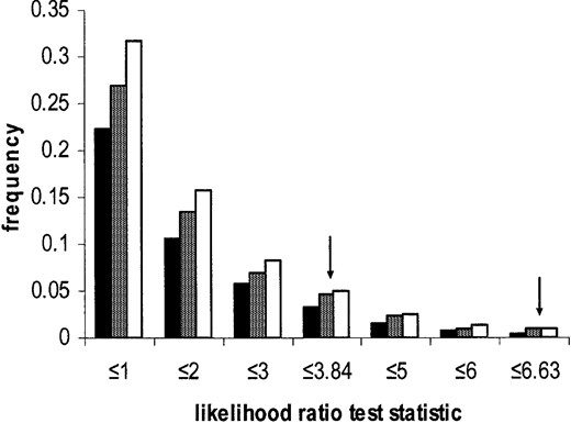
Neutral simulation results studying the behavior of the likelihood-ratio test for selection in the presence and absence of intragenic recombination. Shown is the frequency distribution for the proportion of neutral simulations showing twice the difference in log-likelihoods calculated for the selection model (model 4 in Table 1), allowing selection on locus 10, vs. the neutral model (model 2 in Table 1), assuming free mutation rates across loci. Solid bars are from simulations with intragenic recombination, and shaded bars are with no intragenic recombination. Open bars are the values expected from the χ2 distribution. Arrows show 5% and 1% significance levels.
. Under neutral coalescent simulations with intragenic recombination, the mean and median value of k are close to 1 (mean k = 1.05, median = 0.97), as expected. Furthermore, none of the 1000 simulations shows an estimate of k greater than that observed in this data set (Figure 2)
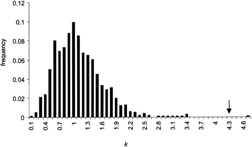
Distribution of the maximum-likelihood estimate of the selection parameter k for locus 10, from 1000 neutral simulations with intragenic recombination. The arrow shows the value estimated for the locus AT1G36310 in the A. lyrata data set.
. Thus, the likelihood method shows significant evidence for a balanced polymorphism at this locus. These results suggest that the likelihood method has higher power than a multilocus HKA test to test for selection at a candidate gene.
To assess the power of the method to detect directional selection, we applied our method to a multilocus data set in maize (Whitt et al. 2002), which compares patterns of diversity for six genes involved in the starch pathway, which have been hypothesized to be under directional selection during domestication, with 11 neutral reference loci. Because of the considerable increase in number of sites per locus (average across loci, 795), the number of segregating sites per locus (average across loci, 26.9), and the divergence (average number of differences between species, 46.5), this analysis took considerably longer to converge (1–10 million chains) and to run (∼17–100 hr on a 2.6-GHz Pentium III computer) in comparison with the A. lyrata data set. We first compare a neutral model, where all 17 loci have k = 1, with a selection model, allowing all six starch pathway genes to be under selection. The likelihood-ratio test is highly significant for this comparison, showing strong evidence for selection on starch pathway genes (Table 3)
Maximum-likelihood analysis of silent polymorphism in the maize data set of Whitt et al. (2002)
k | |||||||||||
|---|---|---|---|---|---|---|---|---|---|---|---|
| Model | Description | ln L | Comparison | Likelihood-ratio statistic (d.f.) | P | bt2 | ae1 | su1 | sh1 | sh2 | wx |
| A | Neutral (all k = 1) | −131.4 | 1 | 1 | 1 | 1 | 1 | 1 | |||
| B | Selection, 3 loci in starch pathway | −110.7 | A vs. B | 32.8 (3) | 3.6 × 10⁻⁷ | 1 | 0.054 | 1 | 0.31 | 0.26 | 1 |
| C | Selection, 6 loci in starch pathway | −110.5 | A vs. C | 32.54 (6) | 1.0 × 10⁻⁵ | 2.0 | 0.04 | 0.93 | 0.46 | 0.24 | 1.87 |
| B vs. C | 0.4 (3) | 0.47 | |||||||||
. However, three of the genes have maximum-likelihood estimates of k that are either close to or greater than one, suggesting that only a subset of genes may have been under directional selection. A model that allows only the 3 loci with k < 1 to be under selection is also highly significant in comparison with the neutral model, and the model with 6 selected loci shows no significant improvement to the likelihood in comparison with the three-gene model (Table 3).
As shown using the maize data set, the method can also easily be applied to test for selection on multiple loci, and the program allows for such models to be tested. However, the power of the method relies on the assumption that at least one locus in the data set follows the strict neutral assumptions and therefore still requires some a priori selection of candidate genes. With the inclusion of a significant number of neutral loci, the method should be much less sensitive to unusual loci and should incorporate the inherent uncertainty in divergence time from individual loci. This should give the likelihood method much more consistency than using a large number of pairwise tests, which have been shown to be difficult to interpret (Moriyama and Powell 1996).
Although the method appears to be fairly robust to the assumption of no recombination, the power to detect a significant reduction or increase in diversity in a given region is likely to depend on the local rate of recombination and the size of the region analyzed; a signature of natural selection using this method may be unlikely in large sampled regions of high recombination, unless selection is very recent and strong. For these types of data, tests that explicitly analyze variation in patterns of diversity across a region (e.g., Kim and Stephan 2002) would be more appropriate.
In addition to the effects of natural selection, violations from the infinite-sites model, intralocus variation in mutation rates, population subdivision, and recent changes in population size (i.e., population bottlenecks and expansion) could lead to a significant likelihood-ratio test, although the extent to which the variance across loci in the ratio of diversity to divergence would be affected by these violations remains unclear. The problems associated with violations of the assumptions of the standard neutral model are shared with most other tests of selection based on polymorphism data, although in principle the multilocus comparisons associated with the HKA framework should be more robust to such violations than tests based on comparing different aspects of diversity at a single locus (e.g., Tajima 1989; Fay and Wu 2000). One important approach to addressing this question would be to first fit the multilocus data to a demographic or mutation model and then examine the distribution of the likelihood-ratio test statistic under this model. If the fit to the chi-square statistic is found to be poor, then more computationally intensive likelihoods could be estimated using simulated data rather than the given equations above, using the same basic likelihood framework. However, the method may be conservative under some demographic models; for example, population expansion is expected to reduce the variance in diversity across loci, and in this case direct use of the above method may be preferable to avoid the computational requirements of exploring by simulation a vast array of possible demographic models and mutation parameters to reach the maximum likelihoods.
Footnotes
Communicating editor: A. H. Paterson
Acknowledgement
We thank D. Charlesworth for helpful discussion, E. Buckler for providing data, and B. Gaut, P. Andolfatto, and two anonymous reviewers for comments on the manuscript. This research was supported by a Royal Society Professorship to B.C. and a Commonwealth Scholarship to S.W.
References
Fay, J. C., and C.-I Wu,
Hastings, W. K.,
Hudson, R. R., 1990 Gene genealogies and the coalescent process, pp. 1–44 in Oxford Surveys in Evolutionary Biology, edited by J. A. D. Futuyma. Oxford University Press, New York.
Hudson, R. R.,
Hudson, R. R., M. Kreitman and M. Aguadé,
Kim, Y., and W. Stephan,
Kimura, M., 1983 The Neutral Theory of Molecular Evolution. Cambridge University Press, Cambridge, UK.
Kreitman, M.,
McVean, G. A., and J. Vieira,
Metropolis, N., A. W. Rosenbluth, M. N. Rosenbluth, A. H. Teller and E. Teller,
Moore, R. C., and M. D. Purugganan,
Moriyama, E. N., and J. R. Powell,
Tajima, F.,
Takahata, N., Y. Satta and J. Klein,
Wall, J. D.,
Whitt, S. R., L. M. Wilson, M. I. Tenaillon, B. S. Gaut and E. S. t. Buckler,
Wright, S. I., B. Lauga and D. Charlesworth,
