Models of Experimental Evolution: The Role of Genetic Chance and Selective Necessity

Abstract

HISTORY has been termed the “realm of contingencies” (Kracauer 1969), implying that the course of history seldom obeys deterministic laws. The contributions from both chance and necessity in the evolution of life are the subject of experimental evolution. The experimental evolution protocol involves establishing a population of microorganisms under laboratory conditions. In experiments involving bacteria, these are grown at constant temperature in a sugar-rich broth. When using viruses, the host species, commonly a bacterium, is maintained alongside the phage in culture. A small set of the founder population is sampled and reintroduced into an otherwise identical but unpopulated environment. The new population is allowed to grow and this population then contributes to the next sample. The procedure is repeated for several generations (serial passaging). These experiments aim to recreate conditions promoting adaptive radiation. Below we describe some key experiments and results summarizing general findings amenable to analysis with our models.

Lenski and Travisano (1994) propagated 12 populations of Escherichia coli B over 10,000 generations. Each population was founded by a single cell derived from an asexual clone. Populations were cultured in a glucose-limited solution at a constant temperature of 37°. Each day populations were diluted by a ratio of 1:100 into an identical solution in which a new phase of growth and eventual starvation could occur. The experiment was designed to facilitate natural selection in the “test tube,” a design in which the fitness criterion is not specified in advance. This is in distinction to artificial selection where the desired outcome is guided by the investigator. Over the course of 2000 generations there was a significant increase in cell size in all 12 replicates. Furthermore there was a significant increase in fitness quantified as the growth rate of an evolved variant placed in the ancestral population. A consistent result across lineages was that the most rapid change in fitness occurred soon after introduction into the experimental environment, during the first 2000 generations. Each lineage appeared to be approaching independent fitness peaks asymptotically. Lenski and Travisano (1994) interpret the common patterns as results of evolution from a single founder combined with large population sizes, whereas any differences are attributed to chance events during the adaptive evolution.

Papadopoulos  et al. (1999) have analyzed the Lenski and Travisano (1994) data set, searching for the genetic correlates of these results using eight insertion sequences (IS) as molecular probes and testing for diversity with a restriction fragment length polymorphism (RFLP) assay. Their results are as follows. For at least 2000 generations of the experiment the IS signature of the ancestor was maintained in replicate lineages. This corresponds to the phase of most rapid fitness increases. During this time many mutations arose that were not maintained for the length of the experiment but that reached significant frequencies—prior to fixation they were replaced by others. The reconstructed phylogeny of genomic substitutions is unbalanced, a tree topology in which only a small number of lineages persist to the end of the experiment. At least two replicate lineages experienced significantly different rates of genetic substitution but showed no significant difference in their increase in fitness. The diverse rates of genomic substitution across replicate populations remained constant whereas the fitness increments diminished. Finally, fitness increments were greatest early whereas genetic diversity increased most significantly once fitness became asymptotic.

Rosenweig  et al. (1994) initiated populations of E. coli from a single clone and showed that stable polymorphisms arose after long periods of glucose-limited continuous culture. These polymorphisms were caused by differential patterns of secretion and uptake of acetate and glycerol. It was later demonstrated that 6 out of 12 independent replicate populations of E. coli evolved “acetate scavenger” polymorphisms, showing an increased genetic diversity with time and predictable, repeatable changes in both phenotype and genotype (Treves  et al. 1998).

Bull  et al. (1997) adapted replicate lineages of the bacteriophage φX174 to growth at high temperatures in two different virus hosts (E. coli and Salmonella typhimurium) within a chemostat. Starting with an “ancestral” population at 38°, the phage were propagated over several generations through a graded increase of 1° daily, reaching a maximum of 43.5°. Fitness of isolates sampled from the chemostat was estimated as the log₂ increase in phage concentration per hour, that is, the number of phage doublings per hour. Sequencing for each of the replicates was conducted every 10 days. An additional four lines were grown from two isolates sampled from the primary lineages in each of the two hosts. It was observed that the average fitness increase was greatest for the early substitutions in the new environment. The substitution rate remained approximately constant across time. Many of the same substitutions were observed in independent lineages within the same host. When reintroduced into the ancestral host, some lineages were able to reverse the changes, thereby readapting to the original host. Thus extensive convergent and parallel evolution was observed. This pattern of substitution made it impossible to correctly infer the phylogeny of lineages.

Bell and Reboud (1997) performed experimental evolution on Chlamydomonas populations. Replicate populations founded by a single spore were propagated by serial transfer in either light conditions or dark conditions supplemented by sodium acetate. Thus in one environment growth was entirely photoautotrophic and in the other entirely heterotrophic. A “sympatric” treatment was also investigated in which light and dark cultures were mixed after each cycle of growth. Fitness was assayed by isolating spores from each culture and growing them up in either light or dark conditions. It was found that the variance in fitness in dark-adapted lineages was an order of magnitude higher than in light-adapted lineages—in the light all lineages grew relatively well. Furthermore, evolution in the light environment compromised performance in the dark environment and vice versa. Thus there was a cost of adaptation. Interestingly, variance in fitness increased through time in the light-adapted lineages whereas in the dark-adapted lineages variance remained constant or decreased. These results held true in both sympatric and allopatric treatments but were more marked in the latter.

Rainey and Travisano (1998) propagated replicate, isogenic populations of Pseudomonas fluorescens in a spatially heterogeneous environment. The environment consisted of a 25-ml beaker filled with 6 ml of King's medium B. In one lineage the solution was shaken regularly whereas in the other the solution was left standing. In the shaken solution—which disrupts spatial structure—the ancestral morph persisted solitarily. In the standing solution, after 3 days, three dominant and distinct morphs had evolved and persisted for the duration of the experiment. The emergence of different morphologies arose in a fixed order, starting with the ancestral “smooth” morph, followed by the “wrinkly spreader” morph, and finally by a “fuzzy spreader” morph. The order of succession was contingent on the presence of the other morphs, such that the fuzzy spreader could only invade on a background of wrinkly spreaders. Thus frequency-dependent selection combined with the existence of spatial “niches” promoted variation.

Wichman  et al. (1999) evolved populations of φX174 (natural host, E. coli) to growth at high temperatures in a novel host, S. typhimurium. Chemostats were sampled every 24 hr and complete genomes sequenced. Fitness was measured as doublings of phage concentrations per hour at 43°. In one replicate (ID) there was a 4000-fold increase in the number of descendants per hour, while in replicate TX, there was an 18,000-fold increase. High degrees of both parallel evolution and adaptive substitution were observed, but the order of substitutions differed between the replicates. The ID lineage lost its ability to replicate in E. coli whereas TX retained this ability.

From this set of experiments and others on RNA viruses (Novella  et al. 1999; Miralles  et al. 2000) and RNA structure modeling (Huynen 1996; Huynen  et al. 1996), one can extract general patterns of evolution: (1) Early genetic substitutions in a new environment confer the largest fitness increments to a genome, (2) phenotype evolution tends to mirror the evolution of fitness increments, with large changes early, (3) rates of substitution remain approximately constant across generations, (4) there is extensive parallel evolution across lineages evolving on the same host—both in phenotype and in genotype, (5) genetic diversity remains low during the phase of maximum fitness increase and increases once fitness becomes asymptotic, (6) evolution toward greater fitness in one host often but not always reduces fitness in an alternative host, and (7) stochastic (bottleneck effects) or spatial heterogeneity leads to an increase in unique patterns of substitution through time.

In the following sections we present a theoretical framework in which many of the questions and patterns described above can be investigated. We first describe the general model and the equilibrium solution of the model, noting that a spectrum of genetic neighbors is maintained by the dominant genotype at any time. We complete the model description by including stochastic effects, both rare mutations and bottlenecks, demonstrating how these increase variability in the evolutionary trajectory.

Using this model, we find that the behavior of evolutionary systems depends critically on the value of the product Np, the population size times the per locus error rate. When Np is small, the rate of evolution is limited by the chance occurrence of beneficial mutations. In contrast, when Np is large and selection pressures are strong, evolution may proceed rapidly through the best possible point mutations, and the rate-limiting step is the time necessary for each beneficial mutation to sweep through the population. These parameter regimes are akin to the two distinct “dynamics of divergence” investigated by Johnson  et al. (1995). In the final sections of the article we derive the rate of divergence and rate of fitness increase for the case when Np is large and selection is strong, illustrating our approach with an application to the experimental evolution of the bacteriophage φX174.

THE QUASI-SPECIES MODEL

We consider a population of N individuals; the genome of each individual is specified by a sequence of length ν. Each locus or “bit” of this sequence has one of A discrete values. A is thus the number of alleles per locus, such that the total number of unique genome sequences, or genotypes, is given by A^ν. We use the term “alleles” here loosely, often setting A = 2 in our simulations for simplicity; more realistic values of A might be 4 (nucleotides) or 20 (amino acids).

We assign a unique fitness, β_i, to the ith genotype. For example, we may consider the case when sequence i is the “wild-type” genome, and all mutations are deleterious: β_j < β_i, ∀j ≠ i. Or we may allow that a few rare mutations increase the fitness of the wild type, either independently or with some sort of epistasis. In the sections that follow, we illustrate several possible models for the distribution of the β_i values.

To integrate Equation 2 deterministically, we set y_i = 0 whenever the frequency of genotype i falls below one individual in the population, or 1/N. Likewise, if the frequency y_i is equal to zero at any time, ẏ_i must exceed 1/N before the new genotype will be added to the population. This provides an approximation of the underlying stochasticity, which we treat more formally in a later section.

Equilibrium solution: We can also rewrite Equation 2 in matrix form: βQȳ = Φȳ, where Φ and β are diagonal matrices of Φ and the β_i, respectively, ȳ is a vector of the y_i, and Q is the matrix with Q _ij in the ith row and jth column. The equilibrium of the system will then be given by the eigenvector corresponding to the largest eigenvalue of βQ.

If the β_i are distinct, a unique stable equilibrium will exist, in which the genotype with the highest β_i dominates the system (Thompson and McBride 1974; Jones 1978). If the population size is sufficiently large and the mutation rate is low compared to the genome length (1 – q < 1/ν), a spectrum of other genotypes that are genetic neighbors of the dominant genotype will be maintained at low frequencies by the mutation-selection balance. This equilibrium state may not, of course, be accessible from all starting points, since some of the “steps” on the evolutionary trajectory may involve genotypes with low fitness or initial frequencies that would be much less than 1/N. This situation can be better modeled by allowing rare mutations to occur probabilistically, as described in the following section of the article. Finally, we note that even when the system is not in equilibrium, any high frequency genotype will continually create a suite of low frequency genetic neighbors. This feature becomes important in later sections.

ASSIGNING FITNESS

As an example, consider an eight-bit genome with two possible alleles per locus. This gives 2⁸ = 256 possible genotypes. For simplicity we write the wild-type genome as a sequence of eight zeros, 00000000, and assume that the fitness contribution of each “zero” allele is one-eighth (b_k(0) = 1/ν for all k), such that the wild-type genome has an overall fitness β₀ = 1.

Figure 1 illustrates one possible time course of the evolution of such a system. Here we have chosen the fitness contribution of each mutant “one” allele from a random distribution, but have arbitrarily imposed that mutations at certain loci will reduce the fitness contribution of that locus, while mutations at other loci will slightly increase the fitness contribution. In particular, we set b_k(1) < 1/ν when k ≤ 5 and b_k(1) > 1/ν when k ≥ 6. Thus mutations in the first five bits of the genome are deleterious, while a mutation in bits 6, 7, or 8 gives some (randomly determined) increase in fitness. We start with a uniform population of the wild-type genome at time t = 0 and assume a generation time of 20 min and population size of 10⁷.

Figure 1.

Open in new tabDownload slide

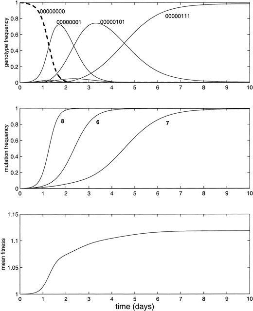
—The evolution of a simple genome. (Top) The frequencies of each genotype in the population, for the simulated evolution of 10⁷ asexual individuals over 10 days. We start with a uniform population of the wild-type genome (eight zeros, dashed line) at time t = 0 and assume a generation time of 20 min and a mutation rate of 10^–5. Mutations in the first five bits of the genome are deleterious, while a mutation in bit 6, 7, or 8 gives an increase in fitness, as described in the text. (Middle) The frequency of each mutation in the population; (bottom) the mean population fitness. In this example mutations accrue successively, starting with the most beneficial single mutation.

The top of Figure 1 shows the evolution of the resulting system. We see that the population frequency of the wild type (dashed line) drops as the frequency of the genotype with a mutation in the eighth locus increases. This genotype is gradually overtaken by the genotype with mutations in the sixth and eighth loci, which in turn is overtaken by the genotype with the highest fitness (loci 6, 7, and 8 are mutated).

The middle of Figure 1 shows the total frequency in the population of mutations at loci 6, 7, and 8. These lines show the probability at each time that a randomly chosen member of the population would have a mutation at the specified locus. The bottom shows the mean fitness of the population, that is, the fitness of each genotype multiplied by its frequency and summed for all genotypes.

It is interesting to note that the variant with the highest fitness, 00000111, is not the first to sweep the population. This is because the probability of creating a three-mutant neighbor of the wild type is low; in this example we have used q = 0.9999, and therefore Q _ij for a Hamming distance of three is ∼1in10¹². For the population size of 10⁷, three-mutant neighbors of the wild type do not exist at the beginning of the simulation. In contrast, all the one-mutant neighbors of the wild type exist after one generation of replication. The fittest one-mutant neighbor is therefore the first to sweep through the population; when its frequency is sufficiently high the two-mutant genotype appears and outcompetes it, followed by the three-mutant genotype.

We also note a characteristic feature of the population fitness function; as illustrated in the bottom of Figure 1, we found that mutations that cause the largest boosts in fitness are the first to sweep the population. This is true whenever (i) fitness contributions are independent and additive and (ii) every one-mutant neighbor of the wild type is likely to exist. This is a result that was previously observed by Tsimring  et al. (1996), using a mean field model in which the one-dimensional distribution of genotype fitnesses was tracked through time, rather than the N-dimensional genotype space. Under these two assumptions, the “best” single mutation is always available as a one-mutant neighbor of the wild type, and the two-mutant neighbor that has the highest growth rate must also have this best mutation plus the second best. This implies that mutations will sweep through the population in a common order—ranked by their fitness contribution. We address this point further in a later section.

Epistasis: In the simulated examples that follow, we often assign fitness to genotypes using independent additive fitness contributions as described above. Obviously, the interaction of genetic loci must be more complicated than this simplified model, and complete independence is unlikely; we consider some possible forms of epistatis in the discussion. We emphasize that the analytical work presented in this article (deriving the rates of substitution and fitness increase) does not necessarily assume the absence of epistasis in the genome.

STOCHASTIC EFFECTS

The model described above is completely deterministic. For a given fitness landscape, defined by the β_i, and a given starting genome, precisely the same evolutionary trajectory would be followed in every trial. To model experimental evolution with greater fidelity, we add two stochastic features to the system: we allow rare mutations to be generated with some small probability, and we use stochastic sampling to model potential “bottlenecks” in the evolutionary process. For example, one such bottleneck may occur during reinoculation of a chemostat, when tubes are changed.

Rare mutations: To allow for the possibility of rare mutations, we relax the condition for the emergence of a new genotype—that the change in the frequency, ẏ_i, must exceed 1/N before the new genotype is added to the population. Instead, we consider the probability that a new genotype is generated within one generation time.

The product Nẏ_i gives the expected value of the number of type i individuals generated in one generation. These individuals might be generated by a large number of independent processes, that is, by mutation from any of the individuals currently replicating in the population. Thus we can imagine some underlying distribution that gives the probability that zero, one, two, or more type i individuals are generated; the mean value of this random variable is Nẏ_i.

When Nẏ_i > 1, genotype i should clearly be added to the simulation. When Nẏ_i < 1, we should in principle generate a random number distributed as the random variable described above, and add 0, 1, 2 (etc.) type i individuals to the simulation accordingly (an exponential distribution with mean Nẏ_i would be an appropriate model, for example). To approximate this process, we instead draw a random number from a uniform distribution and add a single type i individual if Nẏ_i exceeds the value of the random number. Thus we use a random number that is either 0 or 1 to approximate the more complicated distribution described above; we add either 0 or 1 individuals(s) in such frequencies that the same expected value is achieved. This approximation would not be appropriate if, for example, our dynamical system were subject to invasion barriers (minimum frequencies at which new genotypes can invade).

Figure 2 shows the effect of including a stochastic description of rare mutations in the model. In this example, a mutation at either locus 1 or 2 is deleterious, while mutations in locus 3 or 4, or in both loci 1 and 2 together are advantageous. The top shows the results of a strictly deterministic simulation: the simultaneous mutation of loci 1 and 2 is improbable and therefore does not occur. For the simulation shown in the middle, rare mutations occur probabilistically, and eventually the evolving genome finds the “peak” in the fitness landscape.

Stochastic sampling: In experimental models of evolution, it is often necessary for chemostat tubes, media, etc. to be changed at regular intervals. In this case, a sample of the evolving population may be transferred to reinoculate a new system. This sampling may introduce stochastic effects in the evolving system, because genotypes that are rare in the population may be lost during the transfer. Similarly, oversampling of rare genotypes may considerably boost their frequencies after the transfer.

To model such effects, we halt the integration of Equation 2 at regular sampling intervals, producing a simulated population of N individuals with the appropriate genotypic frequencies. We then choose individuals randomly from this population to produce a new starting population (the inoculant) of size fN, for f π [0, 1]. The frequencies y_i in the inoculant can vary markedly from the presample population frequencies, especially when f or y_i is small.

Figure 3 shows three trials of simulated evolution for a six-locus genome. The starting conditions (100% wild type, 000000) and the fitness landscape (mutations in bits three to six confer a fitness advantage) were identical for each simulation. The population of 10⁷ individuals was resampled once per day, producing a new starting population of size 10³. Although the genome with the highest fitness eventually emerges in each of these trials, the evolutionary trajectory from the wild type to the fittest variant is remarkably different. To construct this example we have used an extremely short genome and a severe sampling ratio, 1 in 10⁴. The illustrated effect, however, will be relevant at much gentler sampling ratios, especially if the genome is long and the fitness function complex.

DIVERGENCE AND FITNESS

At what rate does evolution occur in these experimental systems? To answer this question, we consider the rate of divergence, that is, the rate at which the Hamming distance between the original genome and the consensus genome in the population increases. Given the distribution of fitness coefficients, we can also transform this rate of divergence, or substitution rate, into an expected rate of fitness increase.

For a population size N and an error rate (per locus per replication) given by p = 1 – q, the probability that a one-mutant neighbor of the dominant genome is produced in the next generation is Np(1 – p)^ν–¹ ≈ Np, where ν is the length of the genome. We hypothesize that the divergence behavior of the system depends critically on whether Np is greater or less than one.

As an example, consider the experimental evolution of E. coli (Lenski  et al. 1991; Lenski and Travisano 1994) as compared to the experimental evolution of the DNA bacteriophage φX174 (Bull  et al. 1997; Wichman  et al. 1999). For the set of experiments involving E. coli, the effective population size is ∼3.3 × 10⁷, and the error rate per base pair is ∼6 × 10^–10. This gives Np = 0.02; each position along the genome has a 2% chance of being replicated erroneously in each generation. Since there are three possible errors at each locus, each specific one-mutant neighbor of the dominant genotype has <1% chance of being created in each generation. Two-mutant neighbors would be rare (Np²(1 –p)^ν–²/9 ≈ Np²/9 ≈ 10^–12).

Examining the substitution rate for systems such as this, where Np < 1, Gerrish and Lenski (1998) have demonstrated that the competition between a number of sequentially arising beneficial mutations may interfere with the progression of a given mutation to fixation. This “clonal interference” increases the time between fixation events and slows adaptation (Miralles  et al. 1999).

Figure 2.

Open in new tabDownload slide

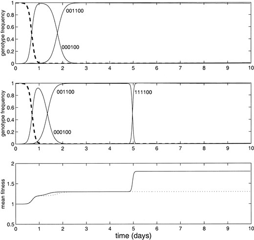
—The effect of allowing rare mutations. (Top and middle) The frequencies of each genotype in the population, for the simulated evolution of 10⁷ individuals over 10 days. Again the generation time is 20 min, the mutation rate is 10^–5, and the simulation is seeded with a uniform population of the wild-type genome (six zeros, dashed lines). In this example a mutation at either locus 1 or 2 is deleterious, while mutations in loci 3 or 4, or in both loci 1 and 2 together are advantageous. (Top) The results of a deterministic simulation: the simultaneous mutation of loci 1 and 2 is improbable and therefore does not occur. (Middle) Rare mutations occur probabilistically as described in the text. Here the simultaneous mutation of loci 1 and 2 eventually occurs. (Bottom) The mean population fitness for the deterministic simulation (dotted line) and the stochastic simulation (solid line).

For the bacteriophage experiments, however, the population size is similar (10⁷), but the mutation rate is much higher (of the order of 10^–6 or 10^–7). Thus Np ≥ 1; there are perhaps one to three copies of every possible one-mutant neighbor of the dominant genome produced in every generation. (Once again, the probability that a specific two-mutant neighbor is produced is low, about 10^–6 or 10^–8 per generation. Since there are >100 million different two-mutant neighbors, however, we find that 10–100 new two-mutant neighbors might be produced on average per generation.) In this situation, all of the one-mutant neighbors are produced almost simultaneously and are immediately in competition with one another. This differs from the situation considered by Gerrish and Lenski (1998), in which the various one-mutant neighbors of the prevailing genome are thrown up probabilistically over time and compete with one another successively.

When Np > 1, many copies of each mutant are produced in each generation, and there is no real risk of a particular beneficial mutation being eliminated by stochastic drift. Therefore, if any of the one-mutant neighbors of the original genome have a higher fitness than the original, they will immediately grow toward fixation. The stronger the selective pressure, the more likely it is that at least one of the many genetic neighbors of the wild type will carry some small fitness advantage. The rate at which this mutation will then sweep through the population depends on the fitness difference between the fittest one-mutant neighbor (genotype j) and the founding genotype (genotype i), irrespective of the fitness coefficients of the other, less fit, competing mutants. [We see this from Equation 2 where to first order we have $y.j=(1−q)βiyi+βjyj−βiyi$⁠; a fuller derivation appears in the following section.]

When a handful of copies of genotype j first appear, the probability of producing a new mutant during the replication of these individuals is extremely low, equivalent to the probability of producing new two-mutant neighbors of type i. As the number of j individuals increases, however, the probability of producing a one-mutant neighbor of genotype j also increases exponentially. At some point before genotype j reaches fixation (in fact, when the frequency of j individuals exceeds 1/Np), it is moreorless certain that all of the one-mutant neighbors of j have been and are continually being produced. If any of these are fitter than j, they will compete with both j and the remaining population of i and will grow toward fixation.

At this point, we note another critical difference between the Np < 1 and Np > 1 cases. When Np > 1, the new mutants that occur while j is growing toward fixation share the mutation that makes j different from the original sequence. That is, they are more likely (by perhaps three orders of magnitude) to be one-mutant neighbors of j, as opposed to two-mutant neighbors of i, which are unrelated to j. Although it is quite possible that genotype j never reaches fixation because of competition from some fitter variant k, k will carry the mutation that characterizes j to fixation.

Figure 3.

Open in new tabDownload slide

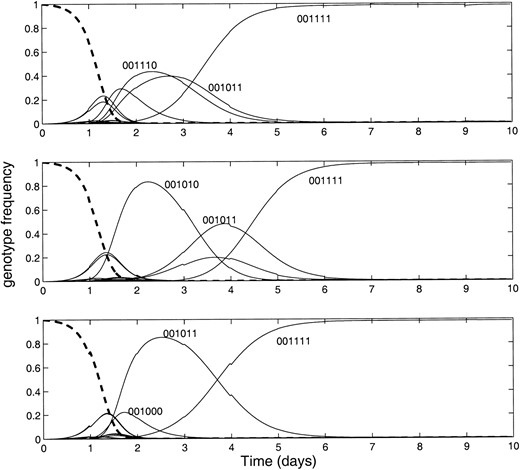
—The effect of stochastic sampling. The genotype frequencies for three separate trials of simulated evolution for a six-locus genome are plotted. All simulations were seeded with a uniform population of the wild-type genome (six zeros). Mutations in bits three to six confer the same fitness advantage in each simulation. Variation in the evolutionary trajectory was introduced by resampling the population of 10⁷ individuals once per day, producing a new starting population of size 10³. Note that the genome with the highest fitness emerges in each of these trials, but the evolutionary trajectory from the wild type to the fittest variant differs markedly. We used a mutation rate of 10^–4 and a 20-min generation time.

Finally, we note that experimentally determined substitution frequencies, deduced from a consensus genotype, follow the fixation time course of individual mutations and not individual genotypes (for example, Wichman  et al. 1999). In the sections that follow, we derive an approximation for the substitution time course of beneficial mutations for systems in which Np > 1.

The increase of a favorable mutation when rare: We are interested in the rate at which favorable mutations are able to sweep through the population, as illustrated in Figure 1. To approximate this rate, we consider the simple case of an asexual population that is dominated by a single genotype, i, and the emergence of a favorable mutation at a single locus. This mutation changes genotype i to genotype j and increases the relative fitness of the genome by an amount s_j. We assume that genotypes i and j are the only genotypes with significantly large frequencies in the population; they are the major players in the population dynamics at this time.

The rate at which new genotypes are accessible: As the frequency y_j increases, the chance that it will produce an erroneous copy of itself increases. As discussed previously, once y_j has exceeded 1/Np, all of the one-mutant neighbors of j are continually being produced by mutation from j. Most of these neighbors will be originally produced at some time before y_j hits this threshold, of course, as the probability Ny_jp approaches 1.

In experimental evolution protocols, the fitness benefit of a point mutation is often remarkably high (for example, s = 3.2–13.9; Bull  et al. 2000; mean s = 0.31; Gerrish and Lenski 1998). These mutations sweep through the population extremely rapidly. Even for a “moderate” fitness increase of 0.31 (a selection coefficient that would still be considered huge in natural evolution), the probability that a one-mutant neighbor of j is produced rises from 0.001 to 1 in ∼20 generations. During these 20 generations, clonal interference will dominate; the currently best mutation will continually be challenged by novel mutant strains. However, this interlude is relatively brief, and it is effectively deterministic: all mutations will be tried and the best is almost certain to win. (During the interlude of clonal interference, a number of mutations will occur probabilistically while y_j « 1/Np. If one of these randomly occurring mutants is much fitter than y_j, it is possible that a point mutation might fix before y_j crosses the 1/Np threshold, i.e., before all the one-mutant neighbors of j have been explored. We assume that this is an unlikely occurrence.)

In reality, there may not be a one-mutant neighbor of j that has a higher fitness than j. In this situation, Np² becomes relevant: if Np² > 1 evolution continues at a rate limited by the accessibility of two-mutant neighbors; if Np² < 1 the system progresses at a rate limited by clonal interference. Along a given evolutionary trajectory, there may be a mix of both types of steps. Whenever one of the one-mutant neighbors of the dominant genotype has any selective advantage, evolution will proceed stepwise through single point mutations; this is very likely the case when the selective pressure is strong. The time between the initial occurrence of the new mutation at each step will then be given by Equation 7, while Equation 6 approximates the time to fixation.

The long-term rate of divergence from the original genotype, however, depends on the distribution of the relative fitness increments, s_i. To estimate these values, we can imagine that 3ν fitness values (corresponding to point mutations in ν positions along the genome and three possible mutations at each position) have been chosen at random from some parent distribution. Suppose s_j = β_j/β_i – 1 is the relative fitness increment of the most fit of these samples. Gillespie (1991) shows that this value is exponentially distributed in the limit as ν approaches infinity, regardless of the initial distribution of fitness values to all possible genotypes. This is because both β_i and β_j are extreme values of the parent distribution. [Gerrish and Lenski (1998) use this model to describe the fitness coefficients of mutations that reach fixation during clonal interference. It is clear that the s_i are even more extreme when Np > 1.]

We demonstrate an application of these formulas in a later section of the article.

Divergence and fitness depend on epistasis: The sections above derive the mean rates of divergence and fitness increase, assuming that the fitness of each new set of one-mutant neighbors is drawn randomly from a set of coefficients with roughly the same distribution. The shape of these curves will be affected, however, by the epistasis between mutations.

Under strong epistasis, the distribution of fitness values among the neighbors of genotype j will have no relation to the distribution around genotype i. In this case the time to fixation will have no correlation with the order in which each mutation appears. In this case, divergence increases roughly linearly at the rate given by Equation 8, while fitness increases exponentially (Equation 10).

Alternatively, if the fitness contributions of each locus in the genome are completely independent and additive (no epistasis), the total fitness for closely related genomes is highly correlated. In this case, beneficial mutations will sweep through the population in order, starting with the “best” mutations. Each new mutant will grow more slowly than the last, times to fixation will grow increasingly long, and the fitness benefit accrued by each successive mutation will be smaller. In this case both divergence, as measured via the consensus genotype, and fitness will be saturating functions, although the mean rates as derived above will still hold.

MODELING THE EVOLUTION OF φX174

As discussed previously, recent experiments involving the bacteriophage φX174 are amenable to analysis using the model proposed here. For example, the derivation of the rate of fitness increase allows for two independent estimates of α, the parameter describing the distribution of fitness coefficients.

Wichman  et al. (1999) report a total increase in fitness from ∼ –5 to 10 doublings per hour, or from 0.32 to 10 individuals per 20-min generation. This increase in fitness was conferred by 13 or 14 nucleotide substitutions and one intergenic deletion, giving a mean fitness increase per substitution of ∼ln(10/0.32)/14 = 0.25, and predicting that α = 4.0. Alternatively, we can use Equation 13, with T = 500 natural generations, N = 10⁷, and p = 10^–7, obtaining α = 4.0. Taking T = 720 (10 days at 20 min per generation) and p = 10^–6 increases our estimate of α to 5.6. The close agreement of these estimates confirms our assumption that the rate-limiting step in this evolutionary trajectory appears to be the rate at which new classes of mutational neighbors are explored. We can use this value of α to compute the median rate of divergence from the original genotype; Equation 8 gives estimates of one substitution every 1–2 days (89 generations).

This estimate of α also allows us to predict the overall divergence and fitness functions, given some assumption about epistasis in the model. Figure 4 (left) compares the estimated divergence rate with the divergence measured in the two experimental trials, assuming independent fitness contributions at each site in the genome. Given that there is only one free parameter, α, which has not been fit to the data illustrated here but has been calculated as described above, the agreement is rather striking. The fact that the observed divergence is slightly faster than predicted could indicate a small degree of nonadaptive substitution; two substitutions may have been nonadaptive according to the analysis of Wichman  et al. (1999). Also, we note that population sizes in the Texas replicate (crosses in Figure 4) were significantly smaller (10⁴) for the first few days of this experiment (Wichman  et al. 1999); this implies that the rate-limiting step for the first several days of evolution would be the waiting time for beneficial mutations to occur, and clonal interference may have posed a delay, offsetting the divergence function.

This offset is also visible when the predicted fitness increase (solid line) is compared with the measured fitness (Figure 4, right). Again we find good agreement between model and measured data, using α = 4 as before.

Figure 4.

Open in new tabDownload slide

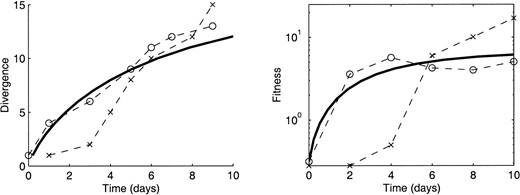
—Measured and predicted divergence in φX174. The total increase in population fitness, the population size, and the mutation rate were used, as described in the text, to estimate a single parameter, α, describing the distribution of relative fitness increments during the evolution of the bacteriophage φX174 (Wichman  et al. 1999). Using this parameter (α = 4), both the divergence (rate of increase in the Hamming distance between the progenitor and the consensus genotype) and the population mean fitness are predicted as functions of time (solid lines). For these estimates we used experimentally determined parameters N = 10⁷, p = 10^–6, η = 15 substitutions and a generation time of 20 min. We assumed that the fitness advantages of the 15 substitutions were evenly spread within the probability distribution p(s) = αe^–αs and made the simplest possible assumption that the benefits of individual mutations are independent (see text for details). These predictions compare well with the results of the ID replicate (open circles), where the population size was roughly constant; small population sizes for the first few days of the TX replicate (crosses) may have delayed the course of evolution. Divergence was determined from the experimental data as the appearance of a new mutation that persisted to the end of the 10-day selection, as seen in Figure 2 of Wichman  et al. (1999); experimental fitness is from Figure 1 of Wichman  et al. (1999).

DISCUSSION

We have demonstrated that the behavior of genetic systems evolving under strong selective pressure may be characterized by the product Np, the population size times the per locus per replication mutation rate. This product is akin to the dimensionless parameter k derived by Johnson  et al. (1995), who first proposed that evolutionary dynamics could be broadly classified into two parameter regimes. When Np is small, the waiting time for a beneficial mutation to occur may be long. When such a mutation does occur, it may be lost through drift or may be outcompeted by a different strain that does not share the same mutation; genetic chance is the rate-limiting step for evolution. This observation has been made by Gerrish and Lenski (1998), who derive a number of characteristic features of such systems for small values of Np, including the expected substitution rate and expected rate of fitness increase.

Alternatively, when Np is large, a substantial number of mutations are produced in every generation. In this case the entire neighborhood of genotype space surrounding the dominant genotype is explored—thoroughly and simultaneously. This corresponds to the “coincident-event collective replacement” described by Johnson  et al. (1995). The stronger the selective pressure, the more likely it is that somewhere in this genetic neighborhood a genotype with some fitness advantage over the wild type exists. The fittest of such genotypes will necessarily outcompete its neighbors, and the rate-limiting step for evolution is the rate at which this genotype takes over the population and begins to explore a new genetic neighborhood. We note that these conditions hold, i.e., selective pressure is strong and Np is large, in a number of systems apart from experimental evolution, including the inhost evolution of human immunodeficiency virus, the evolution of antibiotic resistance, and possibly the development of cancer.

In analyzing the experimental evolution of φX174, we found that the assumption of independent fitness contributions at each locus fit the experimental data very well, particularly for the replicate in which Np was consistently >1. This assumption implies both a high degree of parallel evolution and a conserved order of substitutions, the latter of which was not observed experimentally. We note that the small population size early in one replicate and possible bottleneck effects would be expected to add variability to the genetic trajectory.

It is possible that a small number of mutations could contribute to the same “functional” change in a protein, for example, changing the polarity of some structural element. In this scenario there might be a maximum benefit achieved when all of the relevant amino acids have the appropriate polarity, but a change in one or two may confer a substantial fraction of this maximum benefit. In fact, in any situation where several mutations contribute to the same functional benefit, an epistasis of diminishing returns is likely: the same mutation will confer smaller increases in fitness to fitter genotypes. This effect has been convincingly demonstrated for bacteriophage adaptations to heat (Bull  et al. 2000). In this situation, the fitness benefit of early mutations is, once again, likely to be greater than that of later mutations. Unlike the case of complete independence, however, mutations that confer small increases in fitness may occur early in the mutational sequence if returns are not strictly diminishing.

An alternative way to treat the interaction of genetic loci is through multiplicative fitness contributions (Franklin and Lewontin 1970; Lewontin 1974; Ewens 1979), or through random, additive, nonindependent contributions. The latter model has been studied extensively by Kauffman and colleagues (Kauffman 1993), who found that the fitness benefit caused by early mutations is likely to be greater, on average, than the benefit of later mutations. We emphasize, however, that this is a statistical feature of an epistatically coupled system with a random fitness function, arising simply because more of the genetic “space” has been searched at later times.

Footnotes

Acknowledgement

We thank Jim Bull and Holly Wichman for suggesting that we undertake this project. We gratefully acknowledge the support of The Leon Levy and Shelby White Initiatives Fund, The Florence Gould Foundation, The Ambrose Monell Foundation, The Seaver Institute, and The Alfred P. Sloan Foundation.

LITERATURE CITED