


Abstract
Evolution of multigene families by gene duplication and subsequent diversification is analyzed assuming a haploid model without interchromosomal crossing over. Chromosomes with more different genes are assumed to have higher fitness. Advantageous and deleterious mutations and duplication/deletion also affect the evolution, as in previous studies. In addition, negative selection on the total number of genes (copy number selection) is incorporated in the model. First, a Markov chain approximation is used to obtain formulas for the average numbers of different alleles, genes without pseudogene mutations, and pseudogenes assuming that mutation rates and duplication/deletion rates are all very small. Computer simulation shows that the approximation works well if the products of population size with mutation and duplication/deletion rates are all small compared to 1. However, as they become large, the approximation underestimates gene numbers, especially the number of pseudogenes. Based on the approximation, the following was found: (1) Gene redundancy measured by the average number of redundant genes decreases as advantageous selection becomes stronger. (2) The number of different genes can be approximately described by a linear pure-birth process and thus has a coefficient of variation around 1. (3) The birth rate is an increasing function of population size without copy number selection, but not necessarily so otherwise. (4) Copy number selection drastically decreases the number of pseudogenes. Available data of mutation rates and duplication/deletion rates suggest much faster increases of gene numbers than those observed in the evolution of currently existing multigene families. Various explanations for this discrepancy are discussed based on our approximate analysis.
GENE duplication with subsequent diversification is considered to have played very important roles in the organismal evolution (Ohno 1970, 1988b, 1991). If a gene is duplicated, the selective constraint becomes less for the extra copy, and it can evolve to have a (slightly) different function, while the original function of the gene is kept in the other copy. Thus, gene duplication with subsequent diversification is one of the simplest ways to acquire a new function and is thought to have been employed many times during evolution. For example, Iwabe et al. (1996) suggested that gene duplications contributed to the compartmentalization of a cell and formation of multicellular organisms by creating genes expressed tissue specifically. Also, homeobox genes (Carroll 1995) and MCM1, AGAMOUS, DEFICIENS, and SRF (MADS)-box genes (Thiessen et al. 1996) were apparently created by ancient gene duplications. Gene duplications are not restricted to ancient times. Changes of gene number are observed in closely related species in many taxa, and even examples of polymorphisms with regard to copy number within species are known (e.g., Lyckegaard and Clark 1989; Takano et al. 1989; Lange et al. 1990; Neitz and Neitz 1995). Thus, gene duplications are still ongoing evolutionary processes. How such gene duplications and formation of multigene families occur at the population level is an interesting evolutionary problem.
In the present article, as an extension of Ohta's work, a haploid model of gene duplication is analyzed paying attention to the change of gene number. Copy number selection is explicitly incorporated into the model, and the duplication rate from a single gene was assumed to be 0. First, the model is described. Then, a Markov chain approximation of the model is derived, and its behavior is analyzed assuming low mutation and duplication/deletion rates. Results of extensive computer simulation to check the accuracy of the approximate analysis will be described. Approximate formulas for the rate of increase of the number of different genes and gene redundancy were obtained as a function of population size, mutation rates, duplication/deletion rates, and selection coefficients. Copy number selection was shown to be very effective in reducing the number of pseudogenes. Relationships of various haploid models also will be discussed.
MODEL
Definitions of symbols used are summarized in Table 1. A random-mating haploid population consisting of N chromosomes is assumed. Generations are discrete, and all chromosomes have two identical genes at generation zero. Each chromosome undergoes mutation, gene duplication/deletion, and random sampling with selection, in this order, in one generation.
We call a gene that never has had pseudogene mutation in its descent a live gene. Each live gene mutates to a new different allele or to a pseudogene with rates ua or up, respectively. Here, following the usage of Ohta (1988b), we use the word alleles to denote gene types, although alleles may not be at the same locus. Each new allele is assumed to be different from any other alleles preexisting in the population (Kimura and Crow 1964). Because fitness of a chromosome is a monotone increasing function of the number of different alleles, as described later, ua is the advantageous mutation rate. Once a gene becomes a pseudogene, it stays a pseudogene.
Next, if a chromosome has more than one gene, duplication
Definitions of symbols frequently used in the text
| Symbol | Meaning |
| k | Number of different alleles in a chromosome |
| mi | Number of copies with the ith allelic state |
| n1 | Number of live genes in a chromosome |
| np | Number of pseudogenes in a chromosome |
| nt | Number of total genes in a chromosome |
| N | Population size |
| ua | Mutation rate to a different allele |
| up | Mutation rate to a pseudogene |
| γ | Duplication/deletion rate |
| sa | Coefficient for advantageous selection |
| sd | Selection coefficient for copy number selection |
| f+ | Fixation probability of a chromosome with one more different allele |
| g+ | Fixation probability of a chromosome with one more gene |
| g− | Fixation probability of a chromosome with one less gene |
| α | Rate of increase of the number of different alleles |
| p1(t) | Probability of the population fixed by chromosomes with k = 1 |
| Probability of the population fixed by chromosomes with nt = 1 | |
| R | Ratio of the number of different alleles to the number of pseudogenes |
or deletion occurs with a rate γ/2 per gene copy, respectively. If a chromosome has just one gene, no change occurs. Here, we are considering sister-chromatid unequal crossing over as a genetic mechanism for copy number change. If the mechanism for copy number change is duplicative transposition, copy number change can occur even in chromosomes with a single copy.
Finally, N chromosomes of the next generation are sampled from the N chromosomes of the present generation with probabilities proportional to fitness of each chromosome. Let k and nt be the numbers of different alleles and all genes in a chromosome, respectively. The fitness of the chromosome is zero if k = 0. Otherwise, we consider the following three fitness functions, w(k,nt).
- Model I (Ohta 1987b),where is the average number of different alleles per chromosome in the population, and sa and sd(sa, sd > 0) are positive and negative selection coefficients, respectively.(2)
- Model II (Walsh 1995),(3)
- Model III,Models I and II are modifications of those by Ohta (1987b) and Walsh (1995), respectively, with addition of deleterious effects determined by the total number of genes (copy number selection). As will be noted in the next section, models I, II, and III correspond to the recessive, semidominant, and dominant advantageous mutation models, respectively, in regard to the increase of the number of different alleles. We mainly show results for Model I. Differences among the models will be discussed where relevant.(4)
Random sampling with selection completes one generation. This cycle is repeated many times. At generation zero, the population starts with all chromosomes having two live genes (k = 1, nl = 2, np = 0), and all genes are identical as mentioned before.
Homologous equal crossing over does not occur in the present haploid model. Thus, this is a single locus infinite-allele model. For large populations, the diffusion approximation can be applied, and, in this approximation, relevant parameters are Nua, Nup, Nγ, Nsa, and Nsd measuring time in units of N (Crow and Kimura 1970).
Because the evolution of the model seems very complex, we first analyze a Markov chain whose behavior approximates that of our haploid model under a certain condition. The validity of the approximation will be examined by computer simulation later.
MARKOV CHAIN APPROXIMATION
We assume that Nua, Nup, and Nγ are all very small compared to 1. Also, we assume that positive selection is fairly strong, so that the number of different alleles never decreases. Under these conditions, the population is expected to be mostly monomorphic and thus represented by one chromosome type. A mutant chromosome type that is to replace the currently dominant chromosome type in the population is expected to be fixed quickly. For characterization of a chromosome, let k be the number of different alleles in the chromosome as in the previous section. The chromosome is characterized by k numbers, m1,⋯,mk, each representing the number of live genes with the same allelic state and the number of pseudogenes, np. Thus, in this approximation, the population state is characterized by a vector (m1,⋯,mk,np). The number of live genes, nl, is expressed as , and the total number, nt, is expressed as nt = nl + np. Occasionally, transitions among states occur. Because we assume Nua, Nup, Nγ ≪ 1, one of the following types of changes occurs in a chromosome, and the chromosome is fixed in the population with the probabilities specified below:
- A live gene in the ith class with mi > 1 has an advantageous mutation. The rate of this event is uamiNf+, where f+ is the fixation probability of a mutant chromosome with one more different allele than other chromosomes in the population. Depending on the models of selection, f+ has a different form and is approximately expressed as,where (see Crow and Kimura 1970). Note that the fixation probabilities in models I, II, and III correspond to those of recessive, semidominant, and dominant advantageous mutations, respectively. The derivation for Model III can be done in the same way as that in Model I by Ohta (1987b).(5)
A live gene in the ith class with mi > 1 becomes a pseudogene. Because such change is selectively neutral with mi > 1, the rate for the ith class genes to become a pseudogene is miup.
- The number of live genes of the ith class increases by gene duplication. The rate for this event is miγNg+/2, where g+ is the fixation probability of a deleterious mutant with a selection coefficient −sd and is expressed as (Kimura 1962),(6)
- The number of live genes in the ith allelic class decreases by deletion. The rate for this event in miγNg−/2, where g− is expressed as,(7)
The number of pseudogenes increases by gene duplication. The rate of increase is npγNg+/2.
The number of pseudogenes decreases by deletion. The rate of decrease is npγNg−/2.
The above transition probabilities determine a Markov chain. Because we assumed strong selection (SS) and weak mutation, duplication/deletion (WMD), we call the result of this approximation the SSWMD limit. This type of approximation has been widely used to analyze complex genetic systems (Gillespie 1983; Walsh 1985; Li 1987). In this approximation, further reduction of the number of relevant parameters occurs. If we measure time in units of γ−1, ua/γ and up/γ, in addition to Nsa and Nsd, determine the behavior of the process. The process is still a multidimensional Markov chain and is difficult to analyze directly. So we take two approaches. One is computer simulation of the Markov chain and another is further approximations for studying some
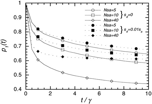
The probability, p1(t), that the number of different alleles is 1 at t. All combinations of Nsa = 5, 10, 40, and sd = 0, 0.01 sa are used for selection coefficients. Other parameters are ua = 0.1γ and up = γ.
aspects of the process. For each parameter set, 10,000 replications were made in the simulation.
Because k is an increasing function of time with strong positive selection, k is always > 1 once k becomes more than 1. We call the phases with k = 1 and k > 1 the first and second phases, respectively. In the first phase, the total number of genes, nt, can become 1, and then no change of the gene number occurs thereafter. For this reason, the number of pseudogenes, np, affects the evolution of k and nt. On the other hand, in the second phase, nl is always larger than 1, and change of the number of genes never stops. The evolution of k and nl does not depend on np. Therefore, these two phases are analyzed separately.
In the first phase, the population starts with k = 1, nt = 2, and we are interested in when the population enters the second phase (k > 1). Let p1(t) be the probability that k is 1 at time t. Because evolution in this phase is influenced by np, p1(t) is difficult to compute. We examined p1(t) by simulation of the Markov chain. Figure 1 shows the time-dependent behavior of p1(t). Solid and broken lines represent results for cases without (sd = 0) and with (sd = 0.01 sa) copy number selection, respectively, and time is measured in units of 1/γ generations. The mutation rates in this example are 10ua = up = γ. The probability p1(t) decreases quickly in the first few 1/γ generations, and then the change becomes small. In the later generations, nt is 1 in most populations with k = 1, and no changes occur in these populations. That is why p1(t) does not change in the later generations. Positive selection decreases the probability, but very weak copy number selection can increase the probability. The effect of copy number selection is stronger for the cases with stronger positive selection.
Ultimately, the population moves to either the state with nt = 1 or that with k > 1. The ultimate probability, p1(∞), was estimated by simulation. Because p1(t) is a monotone decreasing function of t and bounded from the lower side by the probability of nt being 1, simulations are continued until p1(t) − < 0.01 so that we can estimate p1(∞) with a maximum error of 0.01. The results are shown in Table 2. The ratio ua/γ and effects of selection are important in determining p1(∞). For small ua/γ, most populations become ultimately fixed by chromosomes with a single copy. The ratio up/ua has little effect probably because the duplication/deletion force is strong. As ua/γ becomes larger, p1(∞) decreases and the effects of pseudogene mutation become larger. The effect of copy number selection is always significant even though sd/sa = 0.01 in the examples.
In the second phase, we are interested in the evolution of k, nl, and np. We first investigate the ratio Q = nl/k, the average number of genes with the same allelic state and a measure of strict gene redundancy. Because the duplication/deletion process does not stop with nt > 1, the evolution of the number of genes with the ith allelic state, mi (we call this the ith allelic class) can be decoupled from np or other mj's in this approximation. Here, we first concentrate on the evolution of one allelic class and denote the number of live genes in the class by m.
The ultimate probability, p1(∞), of the population being fixed by chromosomes with one copy
| Nsa = 5 | Nsa = 10 | Nsa = 40 | |||||
|---|---|---|---|---|---|---|---|
| ua/γ | up/ua | sd = 0 | sd = sa/100 | sd = 0 | sd = sa/100 | sd = 0 | sd = sa/100 |
| 0.02 | 5 | 0.73 | 0.77 | 0.69 | 0.76 | 0.59 | 0.79 |
| 10 | 0.73 | 0.78 | 0.70 | 0.76 | 0.60 | 0.80 | |
| 0.1 | 5 | 0.54 | 0.58 | 0.49 | 0.55 | 0.38 | 0.54 |
| 10 | 0.58 | 0.62 | 0.53 | 0.60 | 0.42 | 0.61 | |
| 0.5 | 5 | 0.40 | 0.44 | 0.36 | 0.40 | 0.25 | 0.37 |
| 10 | 0.49 | 0.53 | 0.43 | 0.50 | 0.33 | 0.50 | |
Because Mq is the mean number of live genes in one allelic class, its value might be close to the ratio Q = nl/k, although Mq computed above is the equilibrium value. We can check how well Mq can approximate Q by simulation. Because Q is 1 in populations with nt = 1, we computed Q conditioned on nt > 1 from the simulation at t = 10/γ (Table 3). As shown in Table 3, Q estimated from the simulation and Mq computed from (14) agree well. Thus, it seems that the distribution of m is close to equilibrium at t = 10/γ. As Nsa or ua becomes larger, the redundancy measured by Mq becomes less because both b and c increase. Increasing up increases b and thus decreases Mq. Introduction of the copy number selection also decreases Mq. Only when ua/γ is very small, is high genetic redundancy observed, but otherwise the genetic redundancy is very small.
Observed and expected redundancy, Q = nl/k
| Nsa = 5 | Nsa = 10 | Nsa = 40 | ||||||
|---|---|---|---|---|---|---|---|---|
| Sd/sa | ua/γ | up/ua | Obs.a | Exp.b | Obs.a | Exp.b | Obs.a | Exp.b |
| 0.0 | 0.02 | 5 | 2.038 | 1.953 | 1.912 | 1.837 | 1.639 | 1.616 |
| 10 | 1.772 | 1.713 | 1.672 | 1.650 | 1.531 | 1.511 | ||
| 0.1 | 5 | 1.282 | 1.278 | 1.245 | 1.245 | 1.179 | 1.176 | |
| 10 | 1.185 | 1.182 | 1.163 | 1.167 | 1.134 | 1.132 | ||
| 0.01 | 0.02 | 5 | 1.862 | 1.792 | 1.634 | 1.603 | 1.227 | 1.226 |
| 10 | 1.626 | 1.607 | 1.500 | 1.484 | 1.206 | 1.200 | ||
| 0.1 | 5 | 1.257 | 1.254 | 1.206 | 1.205 | 1.097 | 1.094 | |
| 10 | 1.172 | 1.168 | 1.145 | 1.143 | 1.075 | 1.074 | ||
conditioned on nt > 1 at t = 10/7 are computed from the Markov chain simulation.
Mq's computed from Equation 14 are shown.
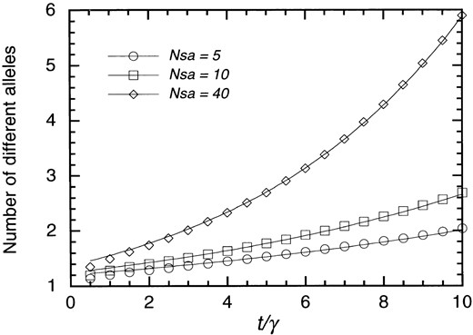
Comparison of the number of different alleles obtained by Markov chain simulation and that expected under a linear pure-birth process. Simulation results are represented by ○, Nsa = 5; □, Nsa = 10; and ♦, Nsa = 40. The curve fits are obtained assuming Equation 17. See text for more detail. Other parameters are ua = 0.1γ and up = γ.
SIMULATION
To examine the validity and limitation of the SSWMD limit obtained by the Markov chain approximation and also to investigate parameter ranges outside that assumed in the approximation, we carried out computer simulation closely following the model. We call this type of simulation the Wright-Fisher simulation. In the simulation, N chromosomes are prepared. In each chromosome, k, m1, …, mk, np and its fitness are stored. Numbers of mutations and duplication/deletion events are determined by generating Poisson random numbers with means computed by multiplying the number of genes and respective rates. Genes undergoing mutations or duplication/deletion are chosen randomly. After these,
Observed and expected number of pseudogenes
| Nsa = 5 | Nsa = 10 | Nsa = 40 | ||||||
|---|---|---|---|---|---|---|---|---|
| Sd/sa | ua/γ | up/ua | Obs.a | Exp.b | Obs.a | Exp.b | Obs.a | Exp.b |
| 0.0 | 0.02 | 5 | 1.119 | 1.102 | 1.237 | 1.228 | 1.469 | 1.490 |
| 10 | 1.650 | 1.667 | 1.840 | 1.822 | 2.312 | 2.308 | ||
| 0.1 | 5 | 3.866 | 3.885 | 4.665 | 4.678 | 6.775 | 6.779 | |
| 10 | 4.093 | 4.127 | 4.679 | 4.734 | 6.797 | 6.869 | ||
| 0.01 | 0.02 | 5 | 0.707 | 0.668 | 0.451 | 0.449 | 0.064 | 0.064 |
| 10 | 1.011 | 0.980 | 0.747 | 0.712 | 0.101 | 0.104 | ||
| 0.1 | 5 | 2.679 | 2.636 | 2.176 | 2.202 | 0.500 | 0.519 | |
| 10 | 2.786 | 2.753 | 2.228 | 2.206 | 0.583 | 0.578 | ||
Values at t = 10/7 are shown.
E[np] computed from the Markov chain simulation.
Values computed from Equation 20 are shown.
the fitness of each chromosome is determined according to (2), (3), or (4) and is divided by the maximum fitness of the current population. The next generation is constructed in the following way: First, choose a chromosome randomly. Next, draw a uniform random number in [0,1) and, if the fitness of the chosen chromosome is less than the random number, add it to the population of the next generation. This is repeated until the chromosome number becomes N. For each parameter set, 1600 replications are made. We present the simulation results in comparison with the SSWMD limit.
First, we examine time courses of the average k, nl, np and the proportion of populations with nt = 1 when Nγ, Nup, and Nua are small and agreement between the Markov chain simulation and Wright-Fisher simulation is expected. Some examples are shown in Figure 3. The values computed by the Markov chain simulation are represented by solid lines and those by the Wright-Fisher simulation are represented by dotted lines. Parameters used are γ = up = 0.001, ua = 0.0001, sa = 0.1, sd = 0, and N = 100 (Figure 3A) and N = 400 (Figure 3B). With N = 100, the Markov chain approximation is very close to the Wright-Fisher simulation. For this parameter set, Nγ = Nup = 0.01 and Nua = 0.001. However, with N = 400, the Markov chain approximation underestimates expected values of k, np, nl by 10 to 20%, especially in the later generations, although they seem to increase exponenetially. The largest discrepancy is found in np. As the number of genes per chromosome increases, the population becomes polymorphic because product parameters such as nlNγ become large. This may be the reason for the discrepancies. Estimates of from the two simulations agree well.
To examine the numbers of genes in a wider parameter range, more simulations were carried out, and some of the results are shown in Table 5 (without copy number selection) and Table 6 (with copy number selection). To clarify the effect of increasing γ, ua, and up, cases with γ = 0.0001 and 0.001 are shown along with the SSWMD limit keeping the ua/γ and up/γ constant. Means and variances of gene numbers at t = 10/γ are shown. With ua/γ = 0.02 and N = 100, values for γ = 0.001 and 0.0001 are quite close to the SSWMD limit. As population size increases (N = 400) or ua/γ approaches 0.1, the values with a large γ (0.001) deviate from the SSWMD limit. Especially, the number of pseudogenes becomes large when γ is large, decreasing the ratio of the number of different alleles to those of pseudogenes. With larger N or ua, populations become polymorphic with regard to gene numbers, thus breaking the assumption of the Markov chain approximation. The increase of pseudogenes is probably due to competition among advantageous alleles and resulting reduction of the probability of fixation of new different alleles. The trend becomes more pronounced when both N and ua are larger (ua/γ = 0.1, N = 400). In this parameter set, the numbers of different alleles and live genes are also larger than the SSWMD limit. This is especially true when there is copy number selection. In the Markov chain approximation, fixations of new alleles are assumed to occur after fixations of redundant copies. However, in polymorphic populations, new, different alleles may appear before fixation of redundant copies. This may increase the fixation rate of new genes, especially when there is copy number selection and fixations of redundant copies are difficult to make occur.
The number of different alleles increases as population size increases without copy number selection. However, this is not necessarily true with copy number selection. With ua/γ = 0.02, the average numbers of different alleles are almost the same for N = 100 and 400. The variance of k is generally very large and in the order of the square of the mean when the mean is large. As ua increases, keeping ua/up constant, E[k] always increases.
Thus far, we investigated only cases with fairly strong selection (Nsa = 10, 40), where one of the assumptions of the SSWMD limit is satisfied. We also investigated when selection is weak, and the result is shown in Table 7.
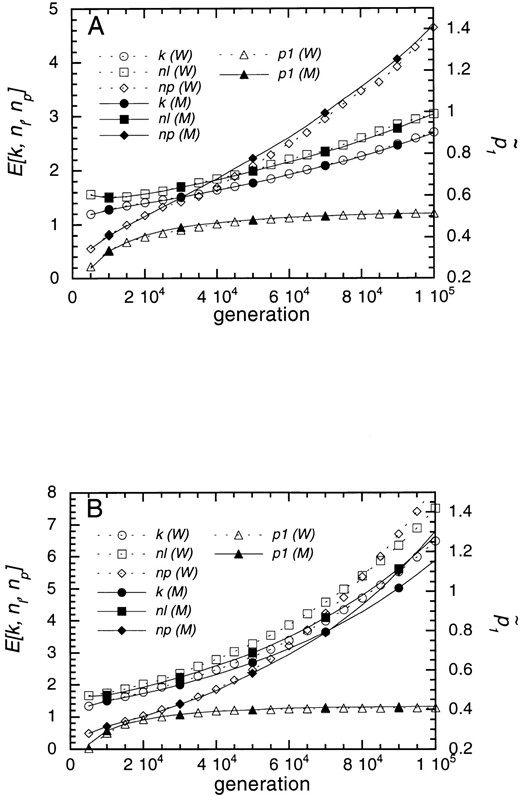
Comparison of the expected numbers of genes obtained by the Markov chain simulation and Wright-Fisher simulation. Two population sizes are used. A, N = 100; B, N = 400. The average numbers of different alleles (k), live genes (nl), pseudogenes (np), and the proportion of populations with nt = 1 (p1) are plotted against generation. Values obtained by the Markov chain simulation (M) are represented by closed symbols with solid lines and those by the Wright-Fisher simulation (W) are represented by open symbols with broken lines. Other parameters are γ = up = 0.0001, ua = 0.00001, sa = 0.1, sd = 0.
The result of reducing γ to 0.0001 was indistinguishable from that of γ = 0.001 and is not shown. The average number of different alleles is very close to 1, although pseudogenes are created. Thus, for smaller populations, new alleles are difficult to evolve. Copy number selection has very little effect on E[k] and slight effects on E[np]. One notable difference from the strong selection case is that E[k] decreases as ua increases, keeping ua/up constant. The effect of increasing up overrides that of increasing ua if Nsa is of the order of 1. Also note that the variance of np is very large. Some populations are considered to have a very large number of pseudogenes, whereas nt = 1 and np = 0 in other populations.
DISCUSSION
In the present article, evolution of multigene families by gene duplication was analyzed assuming a haploid population and no interchromosomal recombination. In such a population, redundant copies are created first, and then one of them evolves to become a new gene by adaptive mutation. This system differs from those in which selection directly operates on the number of gene copies (Ohta 1983; Stephan 1986) in that acquiring adaptive genes requires the presence of redundant genes (Ohta 1987a). To analyze this system, we introduced the Markov chain approximation for small mutation and duplication/deletion rates under which it is assumed that each population is fixed by one chromosome type and that evolution occurs by occasional jumps among chromosome types (the SSWMD limit). By this approximation, the extent of gene redundancy was calculated, and the evolution of the average number of different alleles was characterized. Effects of polymorphism expected under higher mutation and duplication/deletion rates were analyzed using computer simulation. The most significant departure from the SSWMD limit with the same ratios of the rates is the increase of the number of pseudogenes. Also, polymorphism elevates the number of different alleles compared to that computed by the SSWMD limit, especially when there is negative selection on the copy number. With these caveats in mind, we consider some of the questions concerning the evolution of multigene families based on the SSWMD limit.
Numbers of different alleles (k), live genes (n1), and pseudogenes (np)
| k | n1 | np | |||||||
|---|---|---|---|---|---|---|---|---|---|
| ua/γ | N | γa | Mean | Var. | Mean | Var. | Mean | Var. | |
| 0.02 | 100 | 0.001 | 1.611 | 1.699 | 2.301 | 8.034 | 1.799 | 17.737 | 0.6738 |
| 0.0001 | 1.681 | 2.057 | 2.367 | 8.383 | 1.827 | 18.459 | 0.6681 | ||
| M | 1.650 | 2.001 | 2.306 | 8.155 | 1.840 | 18.312 | 0.6748 | ||
| 400 | 0.001 | 2.780 | 8.020 | 4.509 | 32.288 | 3.121 | 34.573 | 0.5825 | |
| 0.0001 | 2.736 | 9.101 | 3.896 | 26.051 | 2.274 | 20.182 | 0.6025 | ||
| M | 2.647 | 8.608 | 3.735 | 23.955 | 2.312 | 21.745 | 0.5960 | ||
| 0.1 | 100 | 0.001 | 2.491 | 4.833 | 2.939 | 8.082 | 5.753 | 73.999 | 0.4894 |
| 0.0001 | 2.729 | 7.932 | 3.095 | 11.501 | 4.906 | 62.177 | 0.5181 | ||
| M | 2.689 | 7.801 | 3.043 | 11.339 | 4.679 | 54.512 | 0.5159 | ||
| 400 | 0.001 | 6.236 | 24.883 | 7.741 | 41.118 | 12.974 | 195.675 | 0.3294 | |
| 0.0001 | 6.624 | 45.713 | 7.595 | 62.824 | 8.187 | 105.184 | 0.3894 | ||
| M | 5.902 | 43.539 | 6.639 | 58.045 | 6.797 | 86.013 | 0.4155 | ||
Values at t = 10/7 are shown. Other parameters are sa = 0.1, sd = 0, and up/ua = 10. Number of replications for each parameter set is 1600.
M denotes the values obtained by the Markov chain simulation.
The increase rate with d = ∞ is γ/2 per generation as expected, but the approach to it is affected by the pseudogene mutation rate. Between these two extreme cases, α* was numerically shown to be an increasing function of d in the range 0.01 ≤ up/γ ≤ 10 (data not shown). Thus, for example, the rate of increase of gene number is larger in larger populations with sd = 0. However, this is not always true when there is copy number selection (sd ≠ 0), as shown in Figure 4. In these cases, as N becomes larger, α* first increases and then decreases. This is because the effect of copy number selection also becomes larger in larger populations. However, as noted in the previous section, the SSWMD limit underestimates the number of different alleles with copy number selection as the change rates (ua, up, and uγ) become larger. Thus, the decrease of the rate as N increases is not as pronounced, as Figure 4 shows in more realistic situations. Indeed, when ua = 10−5, up = 10−4, γ = 10−4, sa = 0.1, and sd = 0.002, corresponding to set 1 in Figure 4, the average numbers of different alleles at the 10/γth generation were 2.048 ± 0.0103 for N = 200 and 1.896 ± 0.081 for N = 800. In summary, the number of different alleles increases as population size becomes large without copy number selection, but this is not necessarily so with copy number selection.
Next, we examine the speed of gene duplication. We measure it by the doubling time of E[k]. It is expressed by log2/[(Mq − q1)uaNf+] and depends on ua, up, γ, Nsa, and Nsd. We do not have reliable estimates for most of the parameters, but some rough calculation under
Numbers of different alleles (k), live genes (nl), and pseudogenes (np) in copy number selection
| k | n1 | np | |||||||
|---|---|---|---|---|---|---|---|---|---|
| ua/γ | N | γa | Mean | Var. | Mean | Var. | Mean | Var. | |
| 0.02 | 100 | 0.001 | 1.419 | 1.147 | 1.792 | 4.161 | 0.774 | 4.689 | 0.7625 |
| 0.0001 | 1.407 | 0.978 | 1.740 | 3.332 | 0.734 | 4.600 | 0.7612 | ||
| M | 1.452 | 1.180 | 1.805 | 3.834 | 0.747 | 4.529 | 0.7464 | ||
| 400 | 0.001 | 1.693 | 2.306 | 2.081 | 5.706 | 0.294 | 0.827 | 0.7556 | |
| 0.0001 | 1.484 | 1.297 | 1.648 | 2.388 | 0.116 | 0.233 | 0.7856 | ||
| M | 1.436 | 1.165 | 1.567 | 2.055 | 0.101 | 0.232 | 0.8021 | ||
| 0.1 | 100 | 0.001 | 2.278 | 4.300 | 2.631 | 7.033 | 3.011 | 25.729 | 0.5694 |
| 0.0001 | 2.283 | 4.808 | 2.541 | 6.764 | 2.172 | 16.809 | 0.5894 | ||
| M | 2.266 | 5.111 | 2.508 | 7.251 | 2.228 | 16.977 | 0.5914 | ||
| 400 | 0.001 | 3.982 | 13.521 | 4.675 | 20.695 | 2.716 | 15.939 | 0.4869 | |
| 0.0001 | 3.114 | 11.480 | 3.376 | 14.438 | 0.827 | 2.729 | 0.5869 | ||
| M | 2.643 | 7.618 | 2.795 | 9.115 | 0.583 | 1.765 | 0.6091 | ||
Values at t = 10/γ are shown. Other parameters are sa = 0.1, sd = 0.01, and up/ua = 10. Number or replications for each parameter set is 1600.
M denotes the values obtained by the Markov chain simulation.
Numbers of different alleles (k), live genes (nl), and pseudogenes (np) with weak selection
| k | nl | np | ||||||
| sd/sa | ua/γ | Mean | Var. | Mean | Var. | Mean | Var. | |
| 0.0 | 0.02 | 1.130 | 0.261 | 1.477 | 2.526 | 1.411 | 13.711 | 0.7719 |
| 0.1 | 1.068 | 0.087 | 1.158 | 0.313 | 2.967 | 33.561 | 0.6656 | |
| 0.01 | 0.02 | 1.145 | 0.301 | 1.439 | 2.105 | 1.289 | 14.155 | 0.7863 |
| 0.1 | 1.056 | 0.076 | 1.126 | 0.244 | 2.245 | 23.901 | 0.7087 | |
Values at t = 10/γ are shown. Other parameters are N = 25, sa = 0.1 and up/ua = 10. Number of replications for each parameter set is 1600.
this model is possible. For up, we may use the null mutation rate measured in Drosophila by Mukai and Cockerham (1977). Averaging over four loci encoding various enzymes, they obtained 1.03 × 10⁻⁵ for the null mutation rate per loci. Estimates of unequal crossing-over rates vary widely. For example, in Drosophila, the duplication rates from a single gene at the ma and ry loci are estimated to be 2.7 × 10⁻⁶ and 1.7 × 10⁻⁴, respectively (Shapira and Finnerty 1986). In maize, the rate per copy is estimated to be in the range 10−4 − 10−3 (Sudpak et al. 1993; Eggelston et al. 1995). Here, we tentatively assume γ = 10−4, taking an intermediate value. Currently, we do not have any estimates for the advantageous mutation rate ua or selection parameters sa, sd, but to get a rough idea, let us assume ua = 10−6, employing the bandmorph mutation rate 1.03 × 10⁻⁶, estimated by Mukai and Cockerham (1977) in Drosophila. With Nsa = 40 and no copy number selection, the doubling time is 8 × 10⁴ generations. Because d* ≪ 1, the doubling time is shown to be roughly proportional to (uaNf+γ)−1 from (24), and reducing ua to one-tenth makes the time about 10 times greater. At any rate, gene
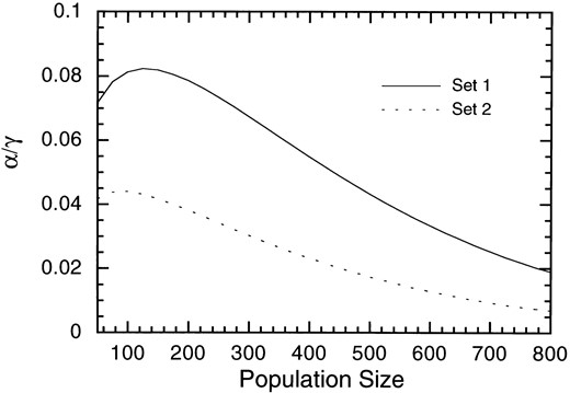
Examples of the rate, α, of increase of the number of different alleles with copy number selection as a function of population size. α/γ is computed from the SSWMD limit as a function of population size. Two examples are shown. Set 1, ua = 0.1γ, up = γ; Set 2, ua = 0.02γ, up = 0.2γ. Other parameters are sa = 0.1, sd = 0.002.
duplications can occur very quickly under the present model from the view point of the evolutionary time scale. However, according to Fryxell (1996), the doubling time is of the order of 10 to 100 million years in a particular lineage of a gene family. Clegg et al. (1997) surveyed three multigene families in plants and estimated new gene recruitment rates to be 2.9 × 10⁻⁸ for Adh, 2.8 × 10⁻⁷ for Chs, and 2.7 × 10⁻⁷ for rbcS. Because explosive gene multiplications are not observed in the evolution of multigene families, Fryxell (1996) proposed that simultaneous coevolution of two or more gene families might be necessary for gene multiplication in respective families, which will diminish duplication rates significantly. However, there are other explanations. For example, Nsa might not be constant. If Nsa becomes close to 1 or less, the number of different alleles stays near 1 as shown by Ohta (1987a,b) and by the present study. Another explanation is copy number selection. If we introduce weak copy number selection (sd = 0.01sa), the doubling times in the above examples become 2 × 10⁶ (ua = 10−7) and 2 × 10⁵ (ua = 10−6) generations, making the times much longer. Thus, copy number selection might have contributed to retarding the duplication rates. Copy number selection might also explain the general observation of larger multiplicity of genes in plants and mammals compared to those in, for example, Drosophila and lower eukaryotes. The numbers of rDNA genes in plants are very large compared to those in Drosophila and seem to contain many pseudogenes (Buckler et al. 1997). The number of pseudogenes is expected to be very small under strong copy number selection (see Tables 4 and 6).
We usually observe large variation in gene numbers in one multigene family among related species. For example, in Drosophila amylase genes, the numbers of genes are two (Payant et al. 1988; Shibata and Yamazaki 1995), one to three (Brown et al. 1990), and at least four (Da Lage et al. 1992) in D. melanogaster, D. pseudoobscura, and D. ananassae, respectively. Such variation can be explained by difference in parameters such as sa and N. However, even with the same parameter set, Clark (1994) showed that multiple equilibrium points concerning gene configuration are possible in two gene systems. Moreover, the variance of gene number is large, an emphasized by Ohta (1987b). As shown here, this is because the increase of gene number behaves like a pure linear-birth process. The coefficient of variation of such a process is asymptotically expressed as , where n0 is the initial number (see p. 159 of Cox and Miller 1965). In our case, a further increase of the variance occurs because the gene number remains 1 in a significant proportion of lineages. Thus, we should expect a very large variance of gene numbers in a multigene family.
In the present article, as a fitness function, Ohta's model (Model I; Ohta 1987b) was mostly used. In the Markov chain approximation, the difference in fitness function contributes only through difference in the fixation probability of a chromosome with one more different allele than other chromosomes in the population. As noted, models I, II, and III correspond to recessive, semidominant, and dominant advantageous mutation models in this regard. Thus, the increase in the number of different alleles is more difficult in this order because a mutant chromosome appears singly at first. However, if we consider a decrease of the number of different alleles by chance, models I, II, and III correspond to dominant, semidominant, and recessive deleterious mutant models. Therefore, although it is most difficult to increase the number of different alleles in Model I, it is also most difficult to decrease it. Dependency on parameters also differes among the models. The fixation rate d = uaNf+/γ of different alleles is proportional to , in Model I and Nsa in Model II (Walsh's model; Walsh 1995). Thus, with the same Nsa > 1, the number of different alleles becomes larger under Model II. For d ≪ 1, α* is proportional to d as shown in (24). Indeed, for Nua = 0.04, Nup = Nγ = 0.4, Nsa = 40, and sd = 0, the Wright-Fisher-type simulation shows that the average number of different alleles at t = 25N was 150 in Model II, whereas it was 6 in Model I. Thus, the selection in Model I is the least efficient in increasing gene number.
We assumed that no duplication/deletion occurs if the total number, nt, of genes becomes 1 because the duplication rate is much smaller if there is only a single copy. We divided the process into the first and second phases, depending on whether k is 1 or more than 1. In the second phase, the evolution is the same as that in Ohta's model (Ohta 1987b). The analysis of the first phase shows that even if Nsa is fairly large, nearly half or more of populations starting from chromosomes with two copies ends up in single gene chromosomes unless ua/γ is not small (Table 2). Thus, we expect to find lineages with only a single gene even if gene number is large in other lineages.
From our approximate analysis, the gene duplication processes in a haploid model without interchromosomal crossing over were characterized, and dependencies of the speed of gene duplication, genetic redundancy, and the number of pseudogenes on various parameters are clarified for strong selection cases. With the accumulation of data on gene families, various discussions on the mechanisms of the evolution of multigene families have been made (e.g., Fryxell 1996; Clegg et al. 1997). Our results will provide a quantitative framework for such discussions by incorporating gene duplication and subsequent divergence into the model. However, higher organisms are mostly diploid, and interchromosomal crossing over does occur. The diploidy and interchromosomal crossing over not included here are known to accelerate the increase of gene number (Ohta 1988a). Incorporating them into the model and analyzing the model in more detail would be necessary for a better understanding of the evolution of multigene families.
Acknowledgement
We thank T. Ohta and M. Iizuka, A. Clark, and an anonymous reviewer for their helpful comments on earlier drafts of the manuscript. This research was partially supported by grants-in-aid to H.T. from the Ministry of Education, Science and Culture of Japan.
Footnotes
Communicating editor: A. G. Clark
LITERATURE CITED
