Establishment of New Mutations in Changing Environments

Abstract

THE process of adaptation depends on the establishment of new beneficial mutations. To be successful, it is not sufficient that mutations simply enter a population; they have to survive an initial phase of strong random genetic drift during which they can be lost. Once a beneficial mutation rises to a sufficiently large number of copies, the strength of drift becomes negligible and selection drives them to fixation or maintains them at intermediate frequency. The probability that mutations survive loss has been called the probability of fixation, the probability of establishment, or the probability of invasion, depending on the context. This probability plays an important role in determining the rate of adaptation of populations (Gillespie 2000; Orr 2000).

Fixation probabilities of beneficial, neutral, or deleterious mutations have been at the core of population genetics theory since the early days of the field. Traditionally, two alternative frameworks have been used: branching processes (Fisher 1922) and diffusion approximations (Kimura 1962). Branching processes allow for the derivation of simple analytical results. Simulations show that these results are accurate, provided the population size is sufficiently large such that N s ≫ 1. The disadvantage of this approach is that it is limited to beneficial and initially rare mutations. Diffusion approximations on the other hand are more powerful and flexible. One can study deleterious or neutral mutations of arbitrary initial frequency. The downside is that it is often impossible to obtain simple analytical results and the underlying assumptions are often less intuitive than in branching processes.

Using branching processes, Haldane (1927) derived his famous result that the probability of fixation of a beneficial mutation is approximately twice its selective advantage. Haldane assumed Poisson-distributed offspring and a small, constant selection coefficient. Later, Haldane’s result was generalized to arbitrary offspring distributions (see Bartlett 1955; Haccou et al. 2005; Lambert 2006).

The impacts of several genetic and ecological factors on the probability of fixation have been investigated (reviewed in Patwa and Wahl 2008). These include the effects of population structure (Whitlock 2003) and spatial heterogeneity (Whitlock and Gomulkiewicz 2005), interference due to selection on linked loci (Barton 1995; Hartfield and Otto 2011) or due to epistatic interaction (Takahasi and Tajima 2005), and changing population sizes (Ewens 1967; Otto and Whitlock 1997; Wahl and Gerrish 2001; Orr and Unckless 2008). In all of these studies, the selection coefficients are assumed constant in time but other aspects of the environment changed over time or space.

Most studies of time-dependent selection have focused on a stationary distribution of selection coefficients, which, at least in a probabilistic sense, can be interpreted as a time-homogeneous case (Jensen 1973; Karlin and Levikson 1974; Takahata et al. 1975; Huillet 2011). Ohta and Kojima (1968) and Kimura and Ohta (1970) studied models with gradual change in selection coefficients. Their derivations are quite general but require solutions to differential equations that can be obtained only in special cases. Using branching processes, Pollak (1966) studied some aspects of the effect of periodically or consistently changing selection coefficients on the probability of fixation.

Two recent articles have investigated the fixation of beneficial mutations when there is an explicit trend in the change of selection coefficients and population sizes. Uecker and Hermisson (2011) study a continuous-time birth–death process with time-dependent parameters and find results for the probability of fixation and the expected time to fixation. Their approach, based on results from Kendall (1948), is general and flexible but typically requires numerical evaluations. Waxman (2011) uses a diffusion approach that assumes arbitrary changes in population size and selection coefficients for a fixed number of generations, after which the environment stays constant. Again, numerical methods are necessary to calculate fixation probabilities. The strengths and weaknesses of these two approaches are discussed in Wahl (2011).

Despite these recent advances, many questions remain unresolved. No analytical results are available for stochastically changing environments if there is trend and autocorrelation. More generally, no simple analytic results are available for general patterns of environmental change. Such results are needed to improve our understanding of the genetics of adaptation and to guide future studies, both theoretical and empirical.

This article presents the first analytical approximation for the probability of establishment in arbitrarily changing environments. The foundation is a novel approach for studying time-dependent branching processes that assumes environmental fluctuations are small but is general otherwise. Temporal fluctuations can be deterministic or stochastic, and the source of variation in the strength of selection and drift is arbitrary. We also allow for different types of offspring distributions in different generations and variation among offspring distributions within generations. Our main result is the generalization of Haldane’s result for the probability of fixation to arbitrary stochastic or deterministic change in environments. We show that probability of establishment is ∼2s_e, where s_e is a weighted average of the selection coefficients across generations. We use this result to calculate the probability of establishment in several biologically interesting cases and compare these approximations to simulations.

Model and Background

Branching process methods have been studied extensively in population genetics (reviewed in Haccou et al. 2005; Patwa and Wahl 2008). Before we present our results we give a brief outline of the basic results needed in our analysis.

We begin by considering an infinitely large population at demographic equilibrium. Generations are discrete and nonoverlapping. A resident allele is fixed and a single mutant allele is introduced at generation 0. Each copy of the mutant allele in the population produces a random number of descendant copies in the following generation (”offspring”) that is independent of the number produced by other mutant copies. We denote the mean number of offspring that a mutant allele leaves in generation n by μ_n and the selection coefficient by s_n = μ_n − 1. (In a haploid population, s_n is the relative fitness advantage of a mutant, while in a randomly mating diploid population, it is the relative fitness advantage of a heterozygote. Because the ultimate fate of the mutation is decided while mutant homozygotes are still rare, we can ignore their fitness.) The variance in offspring produced by a mutant allele is denoted V_n. There are two possible outcomes: the mutant allele dies out or it becomes permanently established. The probabilities of these two events are denoted 1 − p and p, respectively. We call the first outcome extinction and the second outcome establishment.

The sum in Equation 5 is a weighted sum over the temporal change in the environment. Typically, δ_n(x) will be negative if μ_n > μ* and positive if μ_n > μ*. The contribution of δ_n is weighted by ωⁿ. Because ω < 1, earlier generations have more weight than later generations. In addition, it is easy to see that ω increases with decreasing p* (Karlin and Taylor 1975). Consequently, if the probability for fixation is small, a large number of generations will have an impact on the probability of establishment. On the other hand, the fate of new mutations will be decided early for mutations with a high chance of fixation. Let $pn*$ be the probability of survival until generation n in the reference environment. Then, ω is the rate of convergence of $pn*→p*$ (Karlin and Taylor 1975). In that sense, the reference environment is used to quantify the rate at which the contribution of individual generations declines with increasing n.

Note that Equation 5 approximates the probability of establishment for one series of environments, for instance if the change in environmental conditions is deterministic. Deriving the probability establishment in random environments is straightforward. The only random variables in Equation 5 are the δ_n(1 − p*) terms. (Note that δ_n is a random function.) Since the approximation is linear in δ, we can simply replace every δ_n(1 − p*) in Equation 5 by its expectation. This holds for every stochastic process ${δn(1−p*)},nεℕ0+$⁠.

When selection is weak and fluctuations are small, the only aspect of temporal variation that enters the probability of establishment is the effective selection coefficient. Haldane’s classic result is recovered immediately by setting s_n = s. Because the π that determine s_e can be interpreted as probabilities, we can view the effective selection coefficient as a weighted average. Strongest weight is given to the mutant’s fitness in the first generation that it appears, and weights in later generations are given approximately by e^−s*n, where s* is again the selection coefficient in the reference environment. A similar rate appears in Equation 10 of Uecker and Hermisson (2011) (see also Kendall 1948) and in Equations 7 and 12 of Otto and Whitlock (1997).

In the next section we demonstrate that this choice generally yields very accurate results. In few cases, usually when selection is very weak over long periods, better results may be obtained by using a different reference environment. It is a difficult mathematical problem, however, to give a general guideline for the choice of an optimal reference environment.

Examples

We next illustrate how our results can be applied to particular cases of changing environments. In all examples, we compare our analytical approximation for the probability of establishment (Equation 8) to exact results obtained by numerical iteration of (3) and stochastic simulations (see Appendix E for details on the simulation methods). For large populations (>50,000 individuals), results from individual-based simulations coincide with the numerical solution of (3). For the sake of clarity, when the probability of establishment can be obtained numerically, we do not show results from simulations. The R scripts used for the simulations can be found in supporting information, File S1. All numerical results are obtained using Poisson-distributed offspring. Other distributions yield similarly accurate results (data not shown). Unless otherwise stated, we use the time average of selection coefficients (11) and variance in offspring (12) to define the reference environment.

Monotonic change

Most published studies on the genetics of adaptation rely on the idea that ecology and evolution can be decoupled (see Orr 2010 for a review). This separation of timescales may not always be appropriate. Here, we investigate the effect of a gradually changing environment.

Figure 1 shows comparison of (14) with results obtained by numerical evaluation of (3). The behavior of p as a function of κ can be described by distinguishing three different scenarios. If the timescale of selection is much faster than the timescale of temporal change (κ ≪ s; κ < 0.001 in Figure 1), the probability of establishment is determined largely by the initial selection coefficient and is ∼2s₀. If temporal change occurs on a much faster timescale than selection (κ ≫ s; κ > 0.1 in Figure 1), temporal change has very little effect and p ≈ 2s. If environmental change and selection operate on similar timescales (κ ≈ s; 0.001 < κ < 0.1 in Figure 1), p is intermediate between 2s₀ and 2s.

Figure 1

Open in new tabDownload slide

Monotonic change in the environment. Solid curves show the analytic approximation (14), and the dashed curves show the numerical solution of (3). Parameter values are s = 0.01 and (from top to bottom): s₀ = 0.02, 0.015, 0.005, and 0.

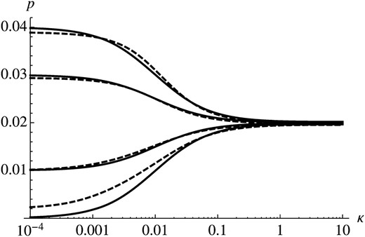
In general, Figure 1 shows that (8) is a very good approximation for the probability of establishment. If s₀ and κ ≪ s, we find, however, that the approximation underestimates the true probability of establishment. The reason for this seems to be that we approximate the decay of the impact of generations by (1 − s*)ⁿ. The exact weight of generation n depends, however, on the history of environments until generation n. Hence, if s₀ and κ ≪ s, we use a timescale of selection that is too fast, which leads to the observed underestimation of p. In this case, a better approximation may be obtained by using a smaller value for s*.

Cyclic variation

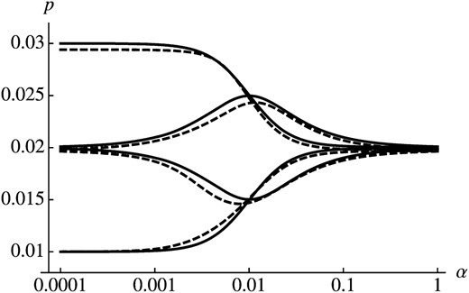
Figure 2 shows comparison of this approximation with numerical calculations. As expected, the initial condition (determined by ϕ) is most important if fluctuations occur on a slower timescale as selection does (⁠$α≪s–$⁠). In contrast, the effect of initial conditions vanishes and the mean selective advantage determines the probability of establishment if $α≫s–$⁠. For $α≈s–$⁠, the dependence on parameters of s_e is more complicated and both α and φ have a strong influence on p (see 0.001 < α < 0.1 in Figure 2).

Figure 2

Open in new tabDownload slide

Periodically changing selection coefficients. Solid curves show the analytic approximation (16) and the dashed curves the numerical solution of (3). Parameter values are $s–=0.01,Δs=0.005$⁠, and (from top to bottom) ϕ = 0, 3π/2, π/2, and π.

Random fluctuations in selection coefficients

Next, we study a stochastic first-order autoregressive model for environmental change: a so-called AR(1) process (Mills and Markellos 2008). Autoregressive processes are commonly used to model time series, for instance, patterns of climate change (Bloomfield and Nychka 1992; Hay et al. 2002).

Figure 3

Open in new tabDownload slide

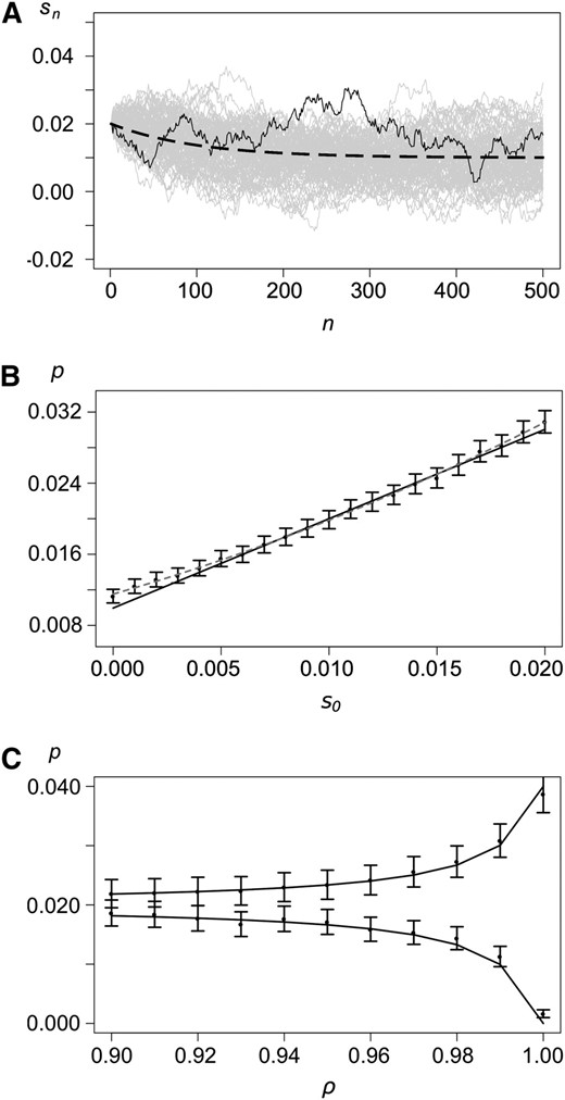
The autoregressive model. (A) Examples of realizations with s₀ = 0.02, $s–=0.01$⁠, σ = 0.001, and ρ = 0.99. The dashed curve shows the mean selection coefficient, and the solid curve shows a single realization. Shaded lines show 50 additional realizations. (B) Probability of establishment as a function of the initial selection coefficient s₀. The solid curve shows the analytical approximation (19), solid dots show results from simulations, and the whiskers show 99% confidence intervals. The shaded dashed line shows the quadratic regression line of the simulated points. Values for the other parameters are as in A. (C) Establishment probability as a function of ρ for s₀ = 0.02 (top) and s₀ = 0 (bottom). Other parameters are as in A.

Variation within generations

So far we have assumed that the numbers of offspring of mutant copies that live in the same generation are independent and identically distributed random variables. It is straightforward to relax the second assumption and extended our results to include variation in the offspring distributions within generations. Such a model accounts for heterogeneity in environmental conditions within a generation (e.g., Levene 1953). An example of the time-independent case can be found in Karlin and Taylor (1975). Here, we briefly discuss the extension to the time-dependent case.

We assume that each copy of the mutant allele has Poisson-distributed offspring. The means of the offspring distributions are drawn independently from an arbitrary distribution with mean $μ–n=1+s–n$⁠. Assuming weak selection, Appendix D shows that the offspring of a randomly drawn copy in generation n is again Poisson distributed and the expected number of offspring is $μ–n$⁠. Consequently, the probability of establishment is given by (8) with $sn=s–n$⁠. As an example, consider normally distributed selection coefficients with mean $s–n=s0e−κn+s(1−e−κn)$ and variance σ². This model is another stochastic version of (13). Figure 4 shows comparison of analytical predictions with simulation results. The example in Figure 4 illustrates that a consistent trend in the average strength of selection has a significant impact on the probability of fixation, even when variance among reproductive successes is large relative to the change in mean selection intensity from one generation to the next.

Figure 4

Open in new tabDownload slide

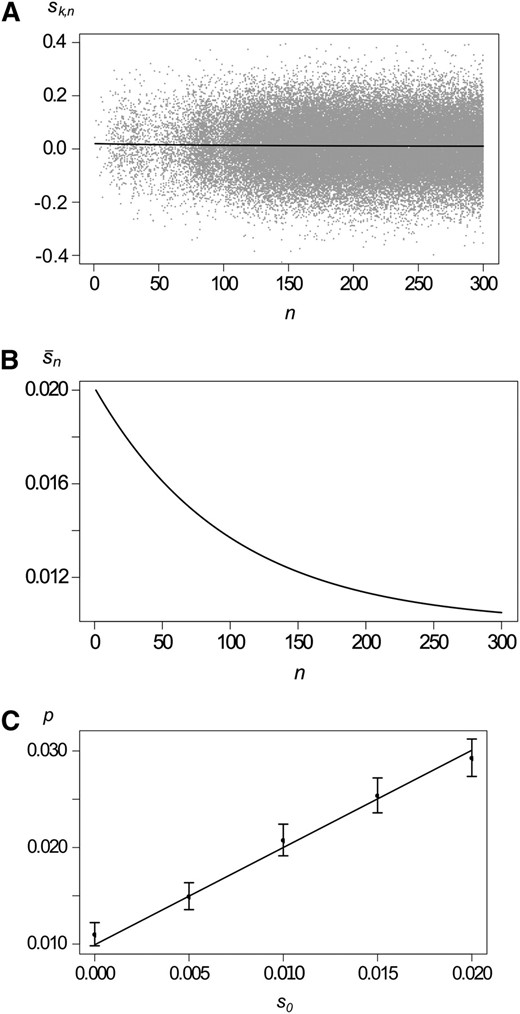
Variation within generations. (A) Illustration of a branching process with variation in offspring distributions within generations. The solid curve shows the mean selection coefficient $s–n$ with κ = 0.01, σ = 0.1, and s₀ = 0.02, and shaded dots show selection coefficients of mutant copies for a single realization. (B) The expected selection coefficient $s–n$ on a different scale. (C) Probability of establishment as a function of the initial selection coefficient s₀. The solid curve shows the analytical approximation, solid dots shows results from simulations, and the whiskers show 99% confidence intervals. Other parameters are as in A.

Changing population size

A comparison of the analytical approximation for p and numerical results is shown in Figure 5. In growing populations (N₀/K < 1), the approximation is very accurate if s and r are of the same order of magnitude. If s ≪ r, however, s_n is large relative to s* in early generations, which causes the approximation to underestimate the true probability of fixation considerably (data not shown). A better approximation can be obtained by using a larger value for s* (see bottom curve in Figure 5). In shrinking populations (N₀/K > 1), s_n will be very small (or negative) during early generations. This causes the approximation to underestimate the probability of establishment if the initial population size is much larger than the carrying capacity. For a more thorough treatment of fixation probabilities in populations of changing size we refer to Otto and Whitlock (1997).

Figure 5

Open in new tabDownload slide

Growing and shrinking populations. Parameter values are s = 0.02, 0.01, 0.01, and 0.001 (from top to bottom) and r = 0.01. In the bottom curve (s = 0.001) we used s* = 0.01 to define the reference environment.

Discussion

The adaptation of a population to environmental challenges is a critical evolutionary process. Sources of environmental variation are manifold and changes can occur on all timescales, ranging from instantaneous changes to transitions on geological timescales. Nevertheless, most studies of the genetics of adaptation rely on a separation of timescales of evolution and ecology (see Orr 2010, for a review). In many cases, this might be a severe oversimplification. Indeed, recent developments on the establishment of beneficial mutations in changing environments reveal that this separation is not always appropriate and can lead to qualitatively different results (see Uecker and Hermisson 2011). Furthermore, the effects on the probability of establishment of trend and autocorrelation have been ignored largely in studies of stochastically changing environments.

This article studies the probability of establishment of beneficial mutations in changing environments. We used an approach that assumes that temporal fluctuations are small, but is general otherwise. The new idea here is to describe the difference of two distributions by the difference of their probability generating functions and perform a perturbation analysis in this function. This approach leads to surprisingly simple yet general results.

Our main result is the generalization of Haldane’s classical result on the fixation of beneficial mutations to arbitrarily changing selection coefficients. Under weak selection, all aspects of environmental variation collapse into a single quantity: the effective selection coefficient s_e. This coefficient is defined as the selection coefficient in a constant environment that leads to the same probability of establishment as the original time-dependent process. The effective selection coefficient s_e is a weighted average over the selection coefficients in each generation, where the weights decrease monotonically over time. Thus the establishment probability is determined by the order in which environments are experienced as well as by their average effect (see Tănase-Nicola and Nemenman 2011 for a discussion of similar findings in deterministic models). The weights are approximately inversely proportional to the expected number of mutants in generation n. This makes sense because the strength of drift will be negligible if the number of mutants reaches a certain threshold (∼1/s*). Consequently, even small changes in selection coefficients from one generation to the next (on the order of s*²) can have a considerable effect on the probability of establishment (cf. Uecker and Hermisson, 2011).

These results apply to beneficial mutations in populations that are large such that $Ns*≫1$⁠. To derive analytical results, we assumed that temporal fluctuations in the offspring distributions are small. A straightforward interpretation of this assumption is difficult because the calculation quantifies the strength of fluctuations using the difference of two probability generating functions. Our results suggest that our approximations hold if fluctuations of selection coefficients are at most of the same order as the strength of selection in the reference environment. This is in agreement with Ohta (1972), who showed that the ratio of mean and variance of selection coefficients can have an important influence on fixation probabilities, especially if this ratio is small.

An important part of our approach is the choice of a suitable reference environment to quantify the fluctuations in reproductive success of mutants. The reference environment should be chosen such that the contributions of the perturbation functions are minimized. It is, however, difficult to give a general guideline for the optimal choice of the reference environment. Indeed, finding a rigorous way to derive the optimal reference environment would be an interesting but challenging subject for future studies. The time average of selection coefficients and variance in offspring seems generally to yield simple and accurate analytical results (see Figures 1–5). When selection is very weak and the environment changes very slowly (relative to the timescale of selection), other choices may yield better results (see s₀ = 0 in Figure 1 and s = 0.001 in Figure 5). As a guideline in experimental settings, our results suggest that one should consider at least 1/s₀ generations to estimate the probability of establishment in changing environments.

To illustrate how the analytical approximations can be used in particular scenarios, we applied them to several biologically interesting cases. In particular, we studied examples of selection changing in consistent, periodical, or random ways. In the latter case, we also studied variation in expected reproductive success among mutant copies within a generation. We also briefly studied mutants with constant selective advantage in populations of changing size. The main focus was on examples with s_n > 0, which ensures that a positive solution of (3) exists. In some examples, however, negative selection coefficients were allowed (see Figures 3–5). These examples illustrate that our approximations can yield accurate results if selection coefficients are negative occasionally (see Figures 3 and 4). In general, however, our approximation underestimates the probability of establishment if s_n ≪ s* for long periods in early generations (see Figures 1 and 5).

Our results shed light on the interaction of environmental and evolutionary dynamics. If the environment changes slowly relative to the timescale of selection, we can separate the timescales of environmental change and evolution (e.g., Orr and Unckless 2008). Conversely, if environmental change occurs at a faster timescale than selection, the mean of the selection coefficients determines the probability of establishment (see Figures 1–3). If selection and temporal change operate on similar timescales, one might naively expect that the probability of establishment is intermediate between the two extreme cases of slow or fast temporal change. Our results illustrate, however, that the dependence on parameters of the effective selection coefficient can be more complicated in such cases (see 0.001 < α < 0.1 in Figure 2). Thus, our results show that separating the timescales of environmental change and evolutionary dynamics is not appropriate if selection and temporal change operate on similar timescales. This conclusion also holds in stochastic environments. Even if expected fitness does not vary over time, autocorrelation can amplify the effect of the initial conditions on the probability of establishment (see Figure 3, B and C). If there is variation in fitness among mutant copies within generations, consistent change in expected selection intensity has a significant effect on the probability of establishment (see Figure 4). This holds even when the variance in fitness within generations is large relative to the change in selection between generations.

The results also reveal implications of environmental change on the distribution of selection coefficients of successful mutations. The timescale of selection is faster for mutations with large effects than it is for mutations with small effects. As a consequence, a consistently degrading environment has a less severe effect on the probability of establishment of mutations with larger effects. This effect is reminiscent of “Haldane’s sieve” (Haldane 1924; Turner 1981), which describes the advantage of dominant beneficial mutations over recessive ones. When environmental stress increases over time, we expect that this “sieve” will be severe and yield an overrepresentation of large mutational effects among successful mutations. Indeed, bias toward large-effect mutations is observed in many cases of adaptation to new environments (Orr and Coyne 1992).

Recent evolution experiments in deteriorating environments (Bell and Gonzalez 2009) led to results consistent with analytical predictions on evolutionary rescue (Gomulkiewicz and Holt 1995; Bell 2008; Orr and Unckless 2008). In these experiments an automated liquid handling system manipulated the selective environment of many hundreds of microbial populations. Such a system could be used to validate a general theory of adaptation and extinction in changing environments. Hence, a general theoretical framework is necessary to formulate broad predictions that can then be tested in experiments. Together with other recent advances (e.g., Campos and Wahl 2010; Uecker and Hermisson 2011), our results illustrate that branching processes are a powerful framework to describe the process of adaptation in changing environments. We hope that our results encourage future work, both theoretically and experimentally, on this important subject.

In summary, we studied the probability of establishment of initially rare beneficial mutations and derived analytical results using a new approach based on the assumption of small temporal fluctuations. Under weak selection, our results are surprisingly simple and provide intuitive insights on the interaction of evolutionary and environmental processes. It would be highly interesting to develop our approach further, e.g., to study the effects of large temporal fluctuations, to calculate approximations for the time until fixation and to allow for correlation in reproductive success among mutant copies.

We close by noting that branching processes have been successfully employed to model many other natural phenomena than the one studied in this work. These include the spread of infectious diseases (e.g., Lloyd-Smith et al. 2005), the growth of tumor cells (e.g., Bozic et al. 2010), and polymerase chain reaction (e.g., Sun 1995). Thus, the ideas we put forward in this study could be useful in a variety of other scientific areas.

Acknowledgements

We thank S. Otto, M. Whitlock, J. Hermisson, and H. Uecker for useful discussions and two anonymous reviewers for helpful comments on the manuscript. This work was funded by National Science Foundation grant DEB-0819901 (to M.K.).

Literature Cited

Appendices

Appendix A: Probability of Survival in a Time-Dependent Branching Process (Equation 3 in the Main Text)

Appendix B: Derivation of Equation 5

Here, we derive an approximation for the probability of establishment if there is no variation in offspring distributions within generations.

Let q_n = Φ_n(0) denote the probability of extinction by generation n. It is straightforward to see that {q_n} is an increasing sequence that is bounded by 1. Intuitively, this can be seen by observing that the probability of extinction in generation n + 1 has to be larger than the probability of extinction in generation n. More formally, it follows because the φ_n are monotonically increasing functions of x. Consequently, q = lim_n→∞  q_n exists and q ε [0, 1]. The probability of establishment is then given by p = 1 − q.

Appendix C: Derivation of Equations 8 and 9

Appendix D: Variation Within Generations

We consider variation in the distribution of offspring among copies of mutant alleles that live in the same generation. Equation A10 shows that the PGF of a randomly drawn mutant copy in generation n is given by $φ–n$ (Equation A8). Note that $φ–n$ is a random function and depends on the particular realization of the process. Hence, we need to calculate the expectation of $φ–n$⁠. In the following, we assume that each copy has Poisson-distributed offspring. The means of these distributions are drawn independently from another distribution that changes over time. Assuming weak selection, we calculate the distribution of the number of offspring of a randomly drawn copy in a given generation.

Appendix E: Simulation Methods

Footnotes

Author notes