Abstract
Recent theoretical studies of the adaptation of DNA sequences assume that the distribution of fitness effects among new beneficial mutations is exponential. This has been justified by using extreme value theory and, in particular, by assuming that the distribution of fitnesses belongs to the Gumbel domain of attraction. However, extreme value theory shows that two other domains of attraction are also possible: the Fréchet and Weibull domains. Distributions in the Fréchet domain have right tails that are heavier than exponential, while distributions in the Weibull domain have right tails that are truncated. To explore the consequences of relaxing the Gumbel assumption, we generalize previous adaptation theory to allow all three domains. We find that many of the previously derived Gumbel-based predictions about the first step of adaptation are fairly robust for some moderate forms of right tails in the Weibull and Fréchet domains, but significant departures are possible, especially for predictions concerning multiple steps in adaptation.
ADAPTATION occurs at the level of DNA sequences. Recent efforts in the theory of adaptation have, therefore, focused on patterns that might characterize the movement of a population through DNA sequence space when evolution is driven by natural selection. Building on Gillespie's seminal work (Gillespie 1983, 1984, 1991), Orr (2002, 2003a, 2005) and Rokytaet al. (2006) derived a number of predictions about the adaptation of DNA sequences. Their models consider the evolution of individual genes and yield predictions that are generally independent of most biological details. In fact, predictions typically depend only on the number of beneficial mutations available to a starting wild-type sequence.
The key assumption underlying this theory is that the distribution of fitness, while unknown, belongs to a large class of probability distributions known as the Gumbel domain of attraction. The Gumbel domain is broad and includes most familiar probability distributions, including the normal, exponential, logistic, and gamma. Extreme value theory shows that the right tails of such distributions have similar behavior. In particular, values in excess of a high threshold are approximately exponentially distributed. In the case of adaptation, then, the distribution of effects among beneficial mutations should be nearly exponential so long as the (unknown) fitness distribution belongs to the Gumbel domain and the wild-type sequence is highly fit (i.e., represents a high threshold).
Although the Gumbel assumption represents a natural starting point for the theory of adaptation, it also represents a possible limitation: extreme value theory shows that non-Gumbel tail behavior can also occur. In particular, extreme value theory shows that a distribution, so long as it meets minimal criteria, can belong to one of three domains: Gumbel, Fréchet, or Weibull. The Fréchet domain loosely corresponds to distributions with heavy tails (heavier than exponential), while the Weibull domain loosely corresponds to distributions with right truncated tails (although the Gumbel domain can also include some right truncated distributions). Although previous workers (e.g., Orr 2006) suggested that the Fréchet and Weibull domains are less natural biologically than the Gumbel, these arguments are far from conclusive. It is therefore important to consider adaptation through DNA sequence space when the Gumbel assumption is relaxed and fitness distributions belong to the Fréchet and Weibull domains. Here we study this problem.
We begin by considering adaptation under extreme forms of the Fréchet and Weibull domains. Though clearly biologically unrealistic, these forms provide valuable intuitions about the more realistic cases that follow. We then derive generalized forms of the results of Orr (2002, 2005) and Rokytaet al. (2006). Most of these general results require introducing only one new parameter, denoted by κ, into the models. By altering the value of κ, we can tune whether the right tail of a fitness distribution behaves like the tail of a distribution belonging to the Gumbel (κ = 0), the Fréchet (κ > 0), or the Weibull (κ < 0) domain.
We find that some of the previous results derived for the Gumbel domain are robust to modest departures into the other domains. Indeed if κ ranges between \({-}\frac{1}{2}\)
and \(\frac{1}{2}\)
, our results are qualitatively similar to those of Orr (2002), who considered κ = 0. We do, though, find qualitatively different patterns of adaptation in the Weibull domain when using parameter values suggested by the empirical work of Rokytaet al. (2008). For some types of Fréchet tails (κ ≥ \(\frac{1}{2}\)
), we obtain unstable results that are difficult to interpret. However, for κ < \(\frac{1}{2},\)
we derive a simple set of results in which findings from Orr (2002, 2005) and Rokytaet al. (2006) represent special cases.
THE MODEL
General assumptions:
We consider a scenario that is identical to that considered by Orr (2002)—a haploid population of DNA sequences of length L adapting under strong-selection weak-mutation (SSWM) conditions; i.e., \(Ns{\gg}1\)
and Nμ < 1, where N is the population size, s is a typical selection coefficient, and μ is the per site per generation mutation rate. Under these conditions, a population adapts through a series of selective sweeps, and the rate of adaptation is limited by the appearance of new beneficial mutations. Also, double mutants occur at too low a rate to influence adaptation; thus only the 3L single-mutant neighboring sequences to the currently fixed sequence need be considered. Deleterious and neutral mutations as well as recombination events are ignored.
The process begins with a population consisting of a wild-type sequence displaced from its fitness optimum, perhaps by an environmental change. If some number of the 3L single-mutant neighbors of this wild type are more fit, then adaptation will occur. If all of the 3L possible mutations and the wild type are ranked by their fitnesses such that the fittest has rank 1, the second fittest has rank 2, etc., then the wild type will have some rank i. Thus i − 1 beneficial mutations are available. One of these i − 1 beneficial mutations will eventually fix in the population, increasing fitness. At this point, the process begins anew.
The generalized Pareto distribution:
To build a model of adaptation, one must posit a distribution for the effect sizes of beneficial mutations. It is safe to assume that the vast majority of mutations available to a wild-type sequence decrease fitness; consequently, beneficial mutations are rare. The classical approach to studying rare events is to consider the upper-order statistics, for example, the maxima of large samples. Extreme value theory shows that the maxima from very large samples converge on one of three possible extreme value distributions (Pickands 1975). Each distribution corresponds to one of the domains of attraction discussed earlier.
Importantly, the distributions for the maximum under all three domains of attraction can be described by a single generalized extreme value distribution (see Embrechtset al. 1997). Results under the special case of the Gumbel domain were used by Gillespie (1991, 1983, 1984) and Orr (2002, 2003a) in their implementations of the model we consider. Specifically, they relied on the distributions of the spacings between the order statistics that have certain convenient properties under the Gumbel domain (in particular, the spacings are independent exponential random variables). Unfortunately, the spacings for distributions in the other two domains lack such simple forms, necessitating an alternative approach.
Our approach is based on the “peaks over threshold” formulation of extreme value theory. This approach considers the distribution of values greater than some high threshold. This approach is natural in the context of adaptive evolution, as we are interested in those mutations that have fitnesses greater than the wild type. If the fitness of the wild type is used as the threshold, the tail of the “excess” distribution describes the distribution of beneficial fitness effects.
In this formulation, the tails of distributions in the three domains of attraction can all be described by the generalized Pareto distribution (GPD) (
Pickands 1975). The cumulative distribution function for the GPD is given by
and its probability density function is given by
In what follows, we use uppercase letters to denote random variables. For example,
S ∼ GPD(κ, τ) means
S is a random variable distributed according to the generalized Pareto distribution with probability density function given by
Equation 2 and
P(
S ≤
s) =
F(
s | κ, τ) given by
Equation 1. We use a lowercase
s to denote a particular observed value of the random variable
S. The parameters in
Equations 1 and
2 are described as follows. The parameter τ determines the scale of the distribution, and κ determines the shape. More precisely, if
Z ∼ GPD(κ, 1) follows the standard GPD (analogous to the standard normal), then
S = τ
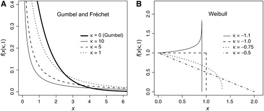
Z is distributed GPD(κ, τ). In this notation, κ > 0 corresponds to the Fréchet domain, κ < 0 corresponds to the Weibull domain, and κ = 0 corresponds to the Gumbel domain (
Figure 1). Note that for the Gumbel domain (κ = 0), the GPD is simply an exponential distribution. Again, if the threshold, which we can (and will) set to zero, is the fitness of the wild type, then the GPD describes the distribution of fitness effects for beneficial mutations.
Rather than rely on properties of the spacings between the upper-order statistics, we instead consider the upper-order statistics themselves from the GPD. If
S ∼ GPD(κ, τ) as in
Equation 1, then
is uniformly distributed on [0, 1]. Then
and thus
S is a decreasing function in
U. If
Uj;i−1 is the
jth smallest value from a sample of size
i − 1 from a uniform distribution, then the corresponding
Sj is the
jth largest value from the GPD. The distributions of the order statistics for the uniform distribution are well known and some relevant properties are provided in
appendix a. Most notably, we make extensive use of the fact that
Uj;i−1 ∼ Beta(
j,
i −
j).
The
lth moment for the GPD exists whenever κ < 1/
l (
Pickands 1975).
appendix b provides a simple way to calculate moments for κ < 0, and the resulting formulas hold for the
lth moment when κ < 1/
l. Thus, if κ < 1 and
S ∼ GPD(κ, τ),
and if κ <
\(1/2\)
, the variance is given by
Higher moments can also be derived and are provided in
appendix b.
RESULTS
We first consider the dynamics of adaptation in terms of fitness ranks. Given an initial wild-type sequence with rank
i, and labeling the selection coefficients of the
i − 1 beneficial mutations as
s = (
s1, … ,
si−1),
Gillespie (1983,
1984,
1991) showed that the probability of moving from the wild-type sequence of rank
i to the beneficial mutation of rank
j is
This assumes the probability that a mutation with selection coefficient
s survives drift is given by Haldane's approximation 2
s (
Haldane 1927) or is at least proportional to
s. We assume that
Equation 7 holds throughout unless stated otherwise.
Orr (2002) showed that if the unknown fitness distribution belongs to the Gumbel domain of attraction, natural selection moves a population on average from initial rank
i to the beneficial mutation with rank
j according to
where the selection coefficients
S = (
S1, … ,
Si−1) are treated as random draws from the tail of a distribution in the Gumbel domain of attraction. Here we generalize this result for fitness distributions in all three domains of attraction. Before deriving the general results, we explore adaptation under this model when κ → −∞ and κ → ∞. Although these extreme cases are clearly not biologically realistic (see below), they provide an intuitive framework for understanding adaptation given more realistic values of κ. They also connect the “move rules” for adaptation that we derive below to those used in other models of adaptation.
Adaptation as κ →−∞:
We first consider the limiting form of the transition probabilities, based on Equation 7, for the Weibull domain as κ → −∞. If S ∼ GPD(κ, τ), then as κ decreases, S becomes less variable. Ultimately, Var(S) → 0 as κ → −∞, as can be seen from Equation 6. Despite this, we will see that Pij(S) converges to the discrete uniform distribution on the integers 1, 2, … , i − 1, which is the most variable of all of the possible distributions for Pij(S).
Suppose
Sj is the
jth largest draw from a sample of size
i − 1 from the GPD(κ, τ) and δ = τ/(1 − κ). If κ → −∞ and τ → −∞ such that δ remains fixed, then the probability density function for
Sj becomes increasingly concentrated at the mean and in the limit is equal to the mean with probability 1. The precise formulation of this limit follows from
Equation A15 in
appendix a and
Equation 4, where we show that
for all
j = 1, 2, … ,
i − 1. Thus, from
Equation 7,
for 1 ≤
j ≤
i − 1.
In words, as κ decreases adaptation becomes more and more random in terms of the identity of the beneficial mutation fixed, although it becomes less variable in terms of the fitness effects [since Var(S) → 0]. In the limit, each beneficial mutation has the same probability of being “grabbed” by natural selection. Interestingly, this “equally often” or “random” move rule has been studied extensively in various models of adaptation, including NK models (Kauffman and Levin 1987; Kauffman 1993) and the block model (Perelson and Macken 1995).
Adaptation as κ → ∞:
In the Fréchet domain, as κ increases, the distribution of
S becomes more variable. In fact, Var(
S) = ∞ for κ ≥
\(1/2\)
. However, we will see that as
S becomes more variable
Pij(
S) becomes less variable, assuming that
Equation 7 holds. From
Equation 4It follows from
Equations A15 and
A16 in
appendix a that
as κ → ∞. We thus find that
In words, the limiting form of adaptation under the Fréchet domain corresponds to “perfect” or “gradient” adaptation, in which the fittest allele is always fixed by natural selection. This move rule has also been well studied in adaptation theory (
Orr 2003b).
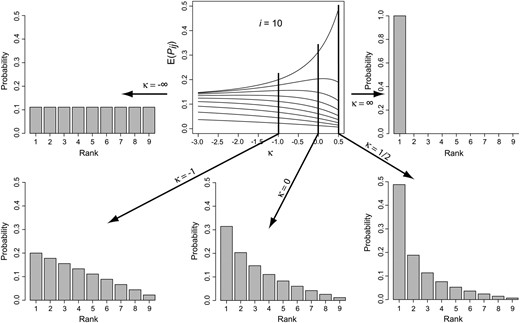
We have thus found that the two extreme (limiting) forms of adaptation correspond to two well-characterized move rules in adaptation: when κ → −∞ (Weibull), evolution gives no preference to any of the more fit alleles and uses a random (i.e., equally often) move rule, whereas when κ → ∞ (Fréchet), evolution uses a perfect move rule. Assuming that Equation 7 holds, adaptation can be viewed as a continuum between random and perfect adaptation with the location along the continuum specified by the shape parameter κ of the GPD (Figure 2). As pointed out by Orr (2002), adaptation under the Gumbel domain (κ = 0) falls exactly between these two extremes (see Figure 2).
Figure 1.—
The three domains of attraction under the generalized Pareto distribution (GPD). (A) The Gumbel domain corresponds to the GPD with κ = 0, and the Fréchet domain corresponds to the GPD with κ > 0. (B) The Weibull domain corresponds to the GPD with κ < 0.
Figure 2.—
Mean transition probabilities from Equation 16 as a function of the shape parameter κ of the GPD. Each curve in the top center plot represents the probabilities for one allele. The top curve provides the probabilities of fixing the allele of rank 1, the next is for the allele of rank 2, etc. The histograms show the transition probabilities for specific values of κ.
Mean transition probabilities in the general case:
To calculate
E(
Pij(
S)) for the general case, we assume
Sj is the
jth largest observation from a sample of size
i − 1 from the GPD(κ, τ). Note that by
Equation 7,
Sj could represent either the
jth largest selection coefficient or the fitness effect. Then by
Equation 4 and by noting
Uj;i−1 ∼ Beta(
j,
i −
j), where
Uj;i−1 is the
jth smallest draw from a sample of size
i − 1 from the uniform distribution on [0, 1] (see
appendix a),
using
Equation 5. We denote the increasing factorial by
x(n) =
x(
x + 1) … (
x +
n − 1) and from
Equation A6 of
appendix a, we find
and thus
Equation 16 is based on a law of large numbers argument that the sample mean
\({\bar{S}}\)
approximates δ, which can be seen in the second line of the derivation of
Equation 14. The validity of this approximation is discussed in detail in
appendix c (
Equation C2 with
r = 1). Although we expect small sample sizes (we are assuming that beneficial mutations are rare), this approximation is quite accurate even for relatively small
i (
Figure 3). The accuracy of the approximation is determined by Var(
S), and as Var(
S) decreases as κ decreases (see
Equation 6), the approximation improves as κ becomes small. Remarkably, this relationship is exact when the
S's are drawn from the exponential distribution. Thus we get perfect argreement with
Equation 8 derived by
Orr (2002) as κ → 0 (see below).
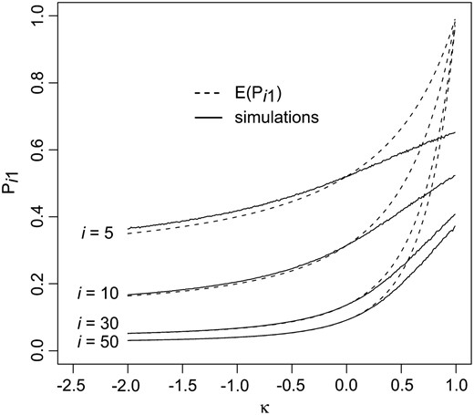
Figure 3.—
The effect of rank of the wild-type i and the shape parameter κ on the accuracy of the law of large numbers approximation used to calculate the mean transition probabilities. The dashed curves represent the probability of fixing the best allele (j = 1) as a function of the GPD shape parameter κ according to Equation 16. The solid lines are simulation results assuming a GPD(κ, 1) with sample size of 10,000. Simulations were performed using R (R DevelopmentCoreTeam 2006).
When evaluated at κ = 0,
Equation 16 yields the indeterminate form 0/0, but we can examine the limit as κ goes to zero. In particular, by
Equations 4,
14, and
16as κ → 0. However, if
U is uniform, then −ln(
U) is exponentially distributed with mean 1, and the
jth largest observation from an exponential has mean
and thus,
where
x(n) =
x(
x + 1) … (
x +
n − 1) is again the increasing factorial. Thus Orr's result,
Equation 8, for the Gumbel domain is recovered.
The jth largest fitness effect Sj will have finite mean only if κ < 1 and finite variance for κ < \(\frac{1}{2}.\)
However, \(P_{ij}(\mathbf{\mathrm{S}}){=}S_{j}/({\sum}_{k{=}1}^{i{-}1}S_{k})\)
is a uniformly bounded random variable, since 0 ≤ Pij(S) ≤ 1. Therefore the expected value of Pij(S) and in fact all of its moments will exist regardless of κ. However, Equation 16 is a valid probability distribution only for κ < 1. For \(\frac{1}{2}\)
≤ κ < 1, the above approximation is extremely poor (Figure 3), as Var(S) is infinite and the law of large numbers approximation fails. For 0 < κ < \(\frac{1}{2}\)
, the approximation is better, though still not good. Equation 16 is plotted in Figure 2 for i = 10 and −3 ≤ κ ≤ \(1/2\)
.
While Equation 16 provides a simple formula for the mean transition probabilities, Equation 14 provides the key insight into their behavior. Equation 14 shows, for example, that when κ = −1, there is a decreasing linear relationship between E(Pij(S)) and U. If κ = −2, there is a quadratic relationship, and when κ = \({-}\frac{1}{2}\)
, there is a one minus a square-root relationship, and when κ = \(\frac{1}{2}\)
, there is a reciprocal of a square root.
Expected rank after a single step:
To fix notation, throughout we assume that the rank of the wild type is
i. We define the distribution of the random variable
Y by
where
E(
Pij(
S)) is given by
Equation 16. Note that
Equation 19 establishes that
Equation 16 reduces to
Equation 8 when κ = 0. Using
Equation 8,
Orr (2002) showed that the expected value of the rank of the allele fixed through natural selection for a population starting at rank
i is given by
Thus a wild type starting at rank 10 will on average be replaced by the third fittest allele. To calculate this in the general case, we assume that
Equation 16 holds and find that for κ < 1
appendix d provides details of this derivation. If κ = 0 then
E(
Y) = (
i + 2)/4, in agreement with Orr's result (
Equation 21 above). If κ ≈ −1, as suggested by
Rokytaet al. (2008), then
E(
Y) = (
i + 1)/3, and
\(\mathrm{lim}_{\mathrm{{\kappa}}{\rightarrow}{-}{\infty}}E(Y){=}i/2\)
. This reflects the move rule noted earlier for this case. When natural selection chooses a mutation randomly it will, on average, reduce fitness rank by one-half.
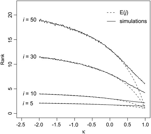
Figure 4 shows
Equation 22 plotted for various values of
i as a function of κ along with simulations. As with the mean transition probabilities, the approximation is poor for κ ≥
\(\frac{1}{2}\)
.
Figure 4.—
The expected fitness rank after a single step in adaptation. The dashed lines give the theoretical expectation according to Equation 22, and the solid lines give the averages of 10,000 simulated data sets. Simulations were performed using R (R DevelopmentCoreTeam 2006).
Orr (2002) showed that for the Gumbel domain (κ = 0), the variance in rank change for a single step in adaptation is given by
An outline of the derivation for the general case is provided in
appendix d. The final result is given by
When κ = 0,
Equation 24 reduces to Orr's result (
Equation 23).
One complete step of adaptation:
After a population substitutes a beneficial mutation through natural selection, it acquires a new set of neighboring sequences. Thus the fitness rank of the new wild-type sequence can change depending on the number of new neighbors that have higher fitnesses. The process through which a new wild-type sequence acquires new neighbors is described in detail by Rokytaet al. (2006) in the case in which the fitness distribution belongs to the Gumbel domain of attraction. To illustrate the idea, consider a sequence of length L = 1000. Initially, the wild-type sequence has some rank, say i = 10; i.e., if the fitnesses of the wild-type sequence and its 3000 single-mutation neighbors are listed in increasing size, the wild type's fitness is 10th from the top. Now assume natural selection moves the population up the list to the sequence having rank Y = 5. The new sequence had rank 5 among the 3001 sequences including the original wild type and its single-mutation neighbors, but now those sequences, except for the original wild type, differ from the new wild type by two mutations and are thus no longer accessible to natural selection. The new wild-type sequence now has a new set of 2999 accessible sequences plus the original wild type and thus, potentially, a new fitness rank. We can imagine that these 2999 sequences are all assigned fitnesses from the same distribution as for the original set and are again listed in increasing order.
Equation 25 below describes the probability distribution for the new rank given that the current sequence had rank
Y in the first set of draws from the fitness distribution. This result is independent of the distribution used to assign fitness, so long as it remains the same for each set of sequences and the rank remains small relative to the number of draws. The asymptotic distribution of the number of values larger than the current fitness in a new sample of fitness values,
i.e., the number of exceedances in a new sample, was derived by
Gumbel and VonSchelling (1950). Assuming 3
L is large, the number of exceedances,
X, has a negative binomial distribution, regardless of the original distribution, such that
where
Y is the starting fitness rank, and
X is the number of draws larger than the current value. It follows from the negative binomial distribution given by
Equation 25 that
E(
X |
Y) =
Y + 1 and Var(
X |
Y) = 2
Y.
Assuming that
X is the rank of the wild type after a single step due to natural selection relative to its new neighbors in sequence space, we find by
Equation 22 that
and by
Equations 22 and
24 that
Probability of adaptation—exact vs. approximate:
In the above sections we assumed that the transition probabilities are given by \(P_{ij}(\mathbf{\mathrm{s}}){=}s_{j}/({\sum}_{k}s_{k})\)
. However, this formula is valid only when s is small and the probability of fixation, denoted by Π(s), is proportional to s. In this section we investigate some of the implications on the theory when the small s approximation does not hold. We consider Π(s) = 1 − e−2s (Kimura 1983) to be a more valid approximation.
We begin by considering
S in the Gumbel domain. That is, we assume that
S is distributed according to the exponential distribution with mean τ. If
F(
s) =
P(
S ≤
s) is the cumulative distribution function for
S, then it follows from elementary probability that
U ≡ 1 −
F(
S) =
e−S/τ is uniformly distributed on the interval [0, 1]. Therefore,
e−2S =
U2τ and Π(
S) = 1 −
e−2S = 1 −
U2τ. Now using the relationship between the uniform distribution and the GPD given by
Equation 4, we get 1 −
U2τ ∼ GPD(−2τ, 2τ). Therefore,
That is, if
S is in the Gumbel domain then the probability of fixation is in the Weibull domain, where the shape and scale parameters have the same magnitude. Thus if the small
s assumption is not valid, then the transition probabilities under the Gumbel domain given by
Equation 8 can be replaced by
Equation 16 with κ = −2τ. However, consider, for example, τ = 0.1. This is a fairly large average selection coefficient and it would be expected that the approximation Π(
s) ≈ 2
s would not hold, but the GPD(−0.2, 0.2) still looks very much like an exponential. So it appears that the results under the Gumbel domain are fairly robust to violations of the small
s assumption. If we apply
Equation 22 with κ = 0.2, we get
E(
Y) = (5 + 3
i)/11; this compares with κ = 0, where
E(
Y) = (
i + 2)/4 = (6 + 3
i)/12. So the mean change in rank is very similar, whether one uses the more accurate probability of fixation or the 2
s approximation.
Under the Weibull domain, \(P({\Pi}(S){\leq}x){=}P(S{\leq}{-}\frac{1}{2}\mathrm{ln}(1{-}x)){=}1{-}(1{-}\mathrm{{\kappa}}\mathrm{ln}(1{-}x)/2\mathrm{{\tau}})^{{-}1/\mathrm{{\kappa}}}\)
, which is only approximately GPD when ln(1 − x) ≈ −x. This distribution is still in the Weibull domain of attraction. However, Martin and Lenormand (2008) showed that to have extreme observations under a right-bounded distribution, the wild type must have fitness fairly close the boundary, which dictates that Π(s) ≈ 2s. Under the Weibull domain it appears that extreme value theory is valid whenever the approximation Π(s) ≈ 2s is valid.
For the Fréchet domain when κ > 1,
E(
S) = ∞ and so it would appear that small
s approximations will certainly not hold. As Π(
s) = 2
s may not be a valid approximation, we again consider Π(
s) = 1 −
e−2s and now we examine the behavior of adaptation as κ → ∞. In
appendix e, we show that if
Sj is the
jth largest draw from a sample of size
i − 1 from the GPD(κ, τ), then
for 1 ≤
j ≤
i − 1. It follows directly that if
\({\Pi}(S_{j}){=}1{-}e^{{-}2S_{j}}\)
is the probability that an allele with fitness
Sj survives drift, then
for 1 ≤
j ≤
i − 1. Thus, the limiting form of the transition probabilities for the Fréchet domain converges to the same limit as for the Weibull domain.
Note that
Equations 13 and
30 lead to conflicting views of the limiting behavior of the transition probabilities under the Fréchet domain. At first glance, it would appear that the conclusion drawn from
Equation 30 is the valid one, as it is based on the more accurate formula for the probability of fixation. However, the limiting transition probabilities in
Equation 30 are valid only if all
Sj are large simultaneously, which is a near impossibility, because the selection coefficient
Si−1 diverges to infinity at a very slow rate, while the largest selection coefficient
S1 diverges very rapidly (see
appendix e). However, it is possible to allow κ → ∞ and still have each
Sj small enough to be biologically relevant, provided we allow τ to vary with κ. An alternative to
Equation 13 would be as follows. Suppose
Sj is the
jth largest draw from a sample of size
i − 1 from the GPD(κ, τ). If κ → ∞ and τ ∝ κ
−κ, then
\(S_{j}{=}(\mathrm{{\tau}}/\mathrm{{\kappa}})(U_{j;i{-}1}^{{-}\mathrm{{\kappa}}}{-}1){\propto}((\mathrm{{\kappa}}U_{j;i{-}1})^{{-}\mathrm{{\kappa}}}{-}1)/\mathrm{{\kappa}}\)
, where
Uj;i−1 is the
jth smallest draw from a uniform distribution. Since (κ
U)
−κ → 0 with probability one (see
appendix e),
Sj → 0 as κ → ∞. Therefore Π(
Sj) ≈ 2
Sj and
Thus, an increasingly heavy-tailed distribution (κ large) with a very small-scale parameter (τ small) has the property that the fittest allele fixes with probability approaching one.
Average fitness improvement for a single step:
Up to this point, we have considered adaptation only in terms of fitness rankings. We now begin to explore the expected behavior of adaptation in terms of fitness effects or, equivalently, selection coefficients. For a single step in adaptation, the population begins with rank
i and beneficial fitness effects
S1,
S2, … ,
Si−1. The population then increases its fitness by Δ
W, which is equal to
Sj with probability
\(S_{j}/({\sum}_{k{=}1}^{i{-}1}S_{k})\)
. By symmetry the results below do not depend on rank order and thus we can treat them as an unordered sample from the GPD. If we assume that
S1, … ,
Si−1 is an (unordered) sample from the GPD(κ, τ), then
Again we assume that the selection coefficients are small enough so that the transition probabilities can be approximated by
\(P_{ij}(\mathbf{\mathrm{S}}){=}S_{j}/({\sum}_{j{=}1}^{i{-}1}S_{j})\)
. Thus, using
Equation 32 and
Equation B5 in
appendix b, we get
Also
Again, using
Equation B5 of
appendix b,
Note that the results of this section do not match Orr's results exactly when κ = 0, but instead provide large
i approximations. For example, if we evaluate
Equation 33 at κ = 0, we get
E(Δ
W) = 2δ. However, the exact result in
Orr (2002) (using our new notation) is
\(E({\Delta}W){=}2((i{-}1)/i)\mathrm{{\delta}}\)
. Note that for κ = 0 the Var(Δ
W) = 2δ
2, which matches only the leading term in
i in Orr's formula,
\(\mathrm{Var}({\Delta}W){=}2\mathrm{{\delta}}^{2}(i{-}1)(i^{2}{+}2)/i^{2}(i{+}1)\)
.
Why do the results in earlier sections match Orr (2002) exactly when κ = 0, while the results of this section only approximate those of Orr (2002) at κ = 0? The distribution of Y is derived using the approximation \(P(Y{=}j){=}(1/(i{-}1))E(S_{j}/{\bar{S}}){\approx}(1/(i{-}1))E(S_{j})/E({\bar{S}})\)
. The validity of this approximation (used in Equation 14) is justified by the law of large numbers and is rigorously established by Equation C2 in appendix c with r = 1. However, it is a remarkable fact that when κ = 0, this is not an approximation, but rather an exact result. This implies that the mean and the variance of the rank distribution E(Y) and Var(Y) agree with the results derived in Orr (2002) when κ = 0. However, in this section we use the approximations \((1/(i{-}1))E(S_{j}^{2}/{\bar{S}}){\approx}(1/(i{-}1))E(S_{j}^{2})/E({\bar{S}})\)
and \((1/(i{-}1))E(S_{j}^{3}/{\bar{S}}){\approx}(1/(i{-}1))E(S_{j}^{3})/E({\bar{S}})\)
, which also follow from Equation C2 in appendix c with r = 2 and r = 3, but are no longer exact results when κ = 0. However, as noted after Equation C2 in appendix c, the above approximations are quite accurate even for small sample sizes. As stated previously, the accuracy of the above approximations is determined by Var(S), and since Var(S) decreases as κ decreases (see Equation 6), the approximation improves as κ becomes small.
The probability of parallel evolution:
Consider two populations that begin with the same wild-type sequence and that have the same set of
i − 1 beneficial mutations. What is the probability that these two populations independently arrive at the
same new sequence at the next step of adaptation? Assuming the distribution belongs to the Gumbel domain,
Orr (2005) showed that this probability = 2/
i. In the general case, let
S1,
S2, … ,
Si−1 be a random sample from the GPD with κ <
\(\frac{1}{2}\)
. Then from
Equation B5 of
appendix b, from
Equation 7, and using the law of large numbers approximation, we find
Thus,
For κ = 0 the result is close to Orr's with
i replaced by
i − 1. The smallest probability occurs when κ = −∞, which corresponds to random adaptation as described above. As κ decreases the probability of parallel evolution decreases, but the decrease is slow and asymptotes to half of what it is in the Gumbel domain.
Mean fitness improvement after multiple steps:
We now compare the average fitness improvement over multiple steps for the Gumbel and Weibull domains. Similar calculations assuming the Fréchet domain are generally not possible, as most of the expectations do not exist (see discussion). In general, for single-step results, the model yields results that change continuously with κ (Figures 2–4). The differences between the domains become much more pronounced when considering multiple steps in adaptation.
If we denote the absolute fitness of allele j by Wj and view it as a random variable from some unknown distribution, then we define the fitness effect of allele j by Wj − Wi, where Wi is the fitness of the wild-type sequence. Selection coefficients are given by (Wj − Wi)/Wi. Recall that in all of the previous results the fitness of the wild type was assumed to be fixed and nonrandom (Wi = wi). Therefore, any result previously derived for selection coefficients involving the GPD(κ, τ) is valid for fitness effects, provided τ is replaced by wiτ. Results that do not depend on the scale parameter τ will be the same under both conventions. However, in this section we view the fitness of the wild type as a random variable, which changes over multiple steps. It is inconvenient to rescale by Wi at each step, and therefore it is more appropriate to deal with fitness improvement. In what follows we admit to a slight abuse of notation. Throughout we use the same notation for fitness effects that was previously used for selection coefficients. We define the fitness effect of the jth fittest allele by Sj ≡ Wj − Wi. If we define δ = E(W − Wi | Wi, W > Wi), then the fitness improvement results above (Equations 33 and 35) still hold.
For the Gumbel domain, because the distribution of beneficial fitness effects is exponential, we can exploit its memoryless property. If fitness effects follow the exponential with mean τ, then the distribution of beneficial effects after the fixation of a beneficial mutation will remain the same. More precisely, if
S is distributed as an exponential with mean τ, then the conditional distribution of
S given
S exceeds
S* is also exponential with mean τ. That is, the new distribution of beneficial fitness effects after substituting a mutation with effect
s \({\ast}\)
is given by
Under the Gumbel domain, the distribution of beneficial effects stays the same after the fixation of a beneficial mutation and does not depend on
s \({\ast}\)
.
This invariance property is only partially true for the GPD. A shifted GPD is still GPD, but unlike the exponential, the scale parameter changes, and the shifted distribution depends on
s \({\ast}\)
. Thus, under the GPD in the Weibull domain (κ < 0), smaller and smaller fitness effects will be observed after each step in an adaptive walk. Thus,
and
E(
S |
S \({\ast}\)
) = (τ + κ
S \({\ast}\)
)/(1 − κ) = δ + (κ
S \({\ast}\)
)/(1 − κ). Assuming the fitness distribution remains the same, the population reaches a new fitness of
Wi + Δ
W. The new distribution of beneficial fitness effects is just the GPD shifted by Δ
W. We denote a random variable with this distribution by
S(1). Denote the original mean fitness relative to
Si as δ
0 instead of δ. Then,
Thus by
Equation 33 we get
Iterating we obtain
Thus, the mean fitness effect decreases to zero geometrically fast in the Weibull domain, whereas in the Gumbel domain the mean fitness effect is invariant under shifts. For example, if κ = −1, then δ
n = δ
0(1/3)
n. Note that Δ
W actually depends on
i and that
Equation 33 is only an approximation. However, the dependence on
i is weak and δ
n would be even smaller if we accounted for
i. The results are, therefore, conservative.
Equations 41 and
42 also hold for 0 < κ <
\(\frac{1}{2}\)
in the Frechét domain, and in this case the mean fitness effects increase geometrically fast.
DISCUSSION
Previous adaptation theory has lived with a certain tension. On the one hand, the theory's most important conclusion is that adaptation is characterized by robust patterns: we can say a good deal about the evolution of DNA sequences independent of knowledge of many biological details (e.g., fitness distribution, gene size, etc.). On the other hand, these conclusions have followed from one major assumption: that the distribution of fitness, while unknown in detail, belongs to the Gumbel domain of attraction. As noted earlier, the Gumbel domain is broad and includes most familiar distributions (normal, exponential, gamma, logistic, etc.). The Gumbel domain also represents the focus of most classical extreme value theory and allows many elegant, closed-form solutions, e.g., to the distribution of spacings between upper-order statistics. For these reasons and others, the Gumbel domain of attraction provides a natural starting point for a theory of adaptation based on extreme value theory. Not surprisingly, Gillespie (1983, 1984, 1991), Orr (2002, 2003b, 2005), and Rokytaet al. (2006) all assumed that the distribution of fitness, while unknown, belongs to the Gumbel domain.
Extreme value theory shows, however, that three domains of attraction are possible for distributions meeting minimal conditions: Gumbel, Fréchet, and Weibull. Although the Fréchet and Weibull domains might first seem less biological than the Gumbel—distributions belonging to the Fréchet domain, in particular, are somewhat exotic, lacking all or higher moments—this impression is obviously far from convincing. Moreover, history suggests caution about casual inferences about the naturalness of various distributions: while early work in mathematical finance often employed Gumbel statistics, data from equity markets now reveal heavy tail distributions of stock returns; i.e., these distributions likely belong to the Fréchet domain of attraction. Analogously, early theoretical work from Gillespie (1984) suggests Gumbel statistics, but empirical data in Rokytaet al. (2008) reject the Gumbel domain in favor of a uniform distribution (κ ≈ −1) in the Weibull domain. It is important, therefore, to study the consequences for the theory of adaptation of departures into the Fréchet and Weibull domains of attraction.
We have studied this problem here. Our approach took advantage of a general version of extreme value theory that encompasses all three domains of attraction. In particular, we analyzed adaptation via the GPD, which provides the distribution of values above a high threshold. (In the case of adaptation, the high threshold represents the fitness of the wild-type allele, while “excesses” above this threshold represent the fitnesses of rare beneficial mutations.) By varying a single parameter, κ, one can “tune” the GPD for the cases of Gumbel, Fréchet, or Weibull domains of attraction.
Our findings show that Gumbel-based results in the genetics of adaptation are often robust to modest departures into the Weibull and, especially, the Fréchet domains of attraction. But in some cases (e.g., κ < \({-}\frac{1}{2}\)
or extended adaptive walks through sequence space), real departures from Gumbel results arise. Because our findings for the Fréchet and Weibull domains also differ from each other, it is worth briefly summarizing our results for these domains separately, emphasizing when they are and are not similar to those for the Gumbel domain.
The Fréchet domain:
Our results for the Fréchet domain are nearly indistinguishable from those of the Gumbel domain, at least in cases that are biologically relevant. Although this finding might at first seem surprising, it can be explained in two different ways. The first involves a simple weak selection approximation. If absolute fitnesses are given by
Wj for 1 ≤
j ≤
i − 1, then the selection coefficients among beneficial mutations are given by
assuming weak selection so that ln(1 +
s) ≈
s. Importantly, if
W belongs to the Fréchet domain, then ln
W is in the Gumbel domain (
Embrechtset al. 1997), and thus our problem reduces to considering the spacings between order statistics for the Gumbel domain. This is the problem that was already addressed by
Orr (2002). We thus arrive at an important conclusion: if selection is weak and a fitness distribution belongs to the Fréchet domain of attraction, the patterns of adaptation will closely resemble those in the Gumbel domain of attraction. This follows immediately from the fact that if
W belongs to the Fréchet domain, ln
W belongs to the Gumbel.
A second way to see why previous Gumbel results are robust to fitness distributions in the Fréchet domain does not involve weak selection. Recall that by
Equation 4 we can express
S in terms of a uniformly distributed random variable such that
\(S{=}(\mathrm{{\tau}}/\mathrm{{\kappa}})(U^{{-}\mathrm{{\kappa}}}{-}1)\)
. If we assume that 0 < κ < 1 so that δ =
E(
S) = τ/(1 − κ) < ∞, then we can rewrite the above to get
\(S{=}(\mathrm{{\delta}}(1{-}\mathrm{{\kappa}})/\mathrm{{\kappa}})(U^{{-}\mathrm{{\kappa}}}{-}1)\)
, which implies that
If κ > 0 is small, we can use the result that ln(1 +
x) ≈
x to say that
and ln(
U) follows the exponential distribution. Note that since the distribution of
S/δ does not depend on δ and has mean equal to one, the above approximation does not require that
S be small. It requires only that κ/(1 − κ) be small enough for the approximation to hold. If the above approximation holds, then
where −τ ln
U follows the exponential distribution with mean τ. Note that
x ≈ ln(1 +
x) is a reasonably accurate approximation for
x as high as 0.4, so the Gumbel domain is robust with respect to moderate departures into the Fréchet domain.
Finally we consider extremely heavy-tailed distributions, i.e., κ > 1. A sample drawn from such a distribution will depend heavily on the scale parameter τ. If the scale parameter is moderate, then the selection coefficient for the fittest allele will be unreasonably large. If the scale parameter is small, then the fitness for the higher ranked alleles will be undetectably small. Therefore, it seems biologically impossible to produce a scenario in which one could draw reasonable inferences under the Fréchet domain that depart significantly from the Gumbel domain. This is one of our most important conclusions.
The Weibull domain:
As pointed out in Rokytaet al. (2008), a right-truncated distribution is not at all unreasonable. For example, even if the phenotypic effects of mutations show no apparent upper bound, the translation of phenotype into fitness might yield a truncated distribution. A pattern of diminishing returns (i.e., a concave mapping of phenotype onto fitness), such as is commonly seen for biochemical reactions (Hartlet al. 1985), could produce an apparent right truncation point for fitness effects, regardless of the underlying distribution of phenotypic effects. Recent theoretical work by Martin and Lenormand (2008) shows that selection to a phenotypic optimum in a “geometric” model of evolution can lead to a Weibull-type distribution of mutational effects, although a Gumbel-type distribution remains a good approximation in the case of many independent characters. There is also empirical evidence from two different viruses to suggest that the Weibull domain may be appropriate in some circumstances (Rokytaet al. 2008).
While the pattern of variability in samples may differ substantially between the Gumbel and Weibull domains, predictions for the first step in an adaptive walk developed by Orr (2002) for the Gumbel domain easily generalize to the Weibull domain (Figure 2). In general, the results describing an average gain after one step are smaller under the Weibull domain than under the Gumbel domain (Figure 3). For example, κ = −1 (as suggested by Rokytaet al. 2008) represents a uniform distribution and κ = 0 represents the exponential distribution. By comparing Equation 21 to Equation 22, we see that the first step in adaptation moves the population on average two-thirds toward the one-step optimum under the uniform model vs. three-fourths under the exponential. Also, using Equation 37 we see that parallel evolution is 1.5 times more likely under the exponential than under the uniform, although both models predict that the probability of parallel evolution is inversely proportional to the rank of the wild type. The mean fitness improvement after one step in adaptation under the exponential distribution is again 1.5 times larger than under the uniform (see Equation 41).
Predictions under the two models differ even more when considering multiple steps. Under the Weibull domain, the mean of the fitness distribution decreases geometrically in the number of steps; i.e., after n steps the mean of the fitness distribution is δn = δ/(1 − 2κ)n. The memoryless property of the exponential distribution, on the other hand, guarantees that the mean of the fitness distribution remains the same after each step.
Much of the present theory of adaptation rests on the assumption of SSWM conditions. However, the geometrically decreasing change in mean fitness suggests that even if SSWM conditions hold during the first step of adaptation, they may fail to do so during later steps. This represents a marked change from results seen under the Gumbel domain.
APPENDIX A: ORDER STATISTICS OF THE UNIFORM DISTRIBUTION
Our results rely extensively on properties of the order statistics of the uniform distribution. Thus, for completeness, we summarize some relevant results. Suppose that
U1,
U2, … ,
Un are independent and identically distributed uniform random variables on the interval [0, 1]. Let
U1;n <
U2;n <
U3;n < … <
Un;n be the order statistics. Thus,
U1;n = min(
U1, … ,
Un) and
Un;n = max(
U1, … ,
Un). If
Uj;n is the
jth smallest observation from a uniformly distributed random sample of size
n, then
Uj;n ∼ Beta(
j,
n + 1 −
j) with density given by
If (
Uj;n,
Ul;n) are the
jth and
lth smallest observations, then their joint density is given by
for 0 <
u <
v < 1 and
j <
l. The conditional distribution of
Uj;n/
Ul;n has the same distribution as the
jth smallest observation from a sample of size
l − 1. Thus,
To see this, note that the conditional density of
Uj;n given
Ul;n is
Let
T =
Uj;n/
Ul;n; then by the standard change of variables formula the conditional distribution of
T given
Ul;n is
implying that the conditional distribution of
T is Beta(
j,
l −
j), which corresponds to the marginal distribution of the
jth smallest observation from a sample of size
l − 1 (see
Equation A1).
From the properties of the beta distribution, the
kth moment of
Uj;n is given by
Note that
and thus from
Equation A6where
x(n) is the increasing factorial
x(n) ≡
x(
x + 1)(
x + 2) … (
x +
n − 1) and Γ(
x) is the gamma function.
APPENDIX B: MOMENTS OF THE GENERALIZED PARETO DISTRIBUTION
Suppose
S ∼ GPD(κ, τ) with density given by
Equation 2 and κ ≤ 0, and
l is any positive integer. If κ = 0, the GPD reduces to the exponential distribution with mean δ =
E(
S) = τ. It can be verified from the exponential distribution that
E(
Sl) =
l!δ
l. For κ < 0, a rescaling of
S gives a beta distribution. If
V = −κ
S/τ, then
V ∼ Beta(1, −1/κ) with density
It follows from properties of the beta distribution that
and
In general,
Thus, if
l is any positive integer and δ =
E(
S) = τ/(1 − κ), then
APPENDIX C: VALIDITY OF THE APPROXIMATION USED TO CALCULATE THE MEAN TRANSITION PROBABILITIES
If
X1,
X2, … ,
Xn are iid random variables with mean δ, variance σ
2, and finite fourth moments, then
The proof of this is a straightforward Taylor series argument that holds for any random sample from any distribution with finite fourth moments. It essentially states that
\(1/{\bar{X}}\)
converges in mean to 1/δ, at the same rate as
\({\bar{X}}\)
converges to δ.
Let
S1,
S2, … ,
Si−1 be rank-ordered observations from a GPD with κ ≤ 0. Then
or for large
i,
where
\(\mathrm{{\varepsilon}}{\approx}1/\sqrt{(1{-}2\mathrm{{\kappa}})(i{-}1)}\)
. Note that the upper bound on the right side of
Equation C2 that establishes the relative error in the approximation
\(E(S_{j}^{r}/{\sum}_{l{=}1}^{i{-}1}S_{l})\)
by
\((1/(i{-}1))E(S_{j}^{r})/E({\bar{S}})\)
is the same for all powers
r.
To derive this result, replace
\(E(S_{j}^{r}/{\sum}_{l{=}1}^{i{-}1}S_{l})\)
with
\((1/(i{-}1))E(S_{j}^{r}/{\bar{S}})\)
and
\(E({\bar{S}})\)
with δ on the left side of
Equation C2, giving
Applying the Cauchy–Schwartz inequality gives
It follows by
Equations 4 and
A12 that
\(\sqrt{E(S_{j}^{2r})}/E(S_{j}^{r}){\rightarrow}1\)
as
i → ∞, and it follows from
Equation C1 that
\((i{-}1)E(1/{\bar{S}}{-}1/\mathrm{{\delta}})^{2}{\rightarrow}\mathrm{Var}(S)/\mathrm{{\delta}}^{4}{=}1/(1{-}2\mathrm{{\kappa}})\mathrm{{\delta}}^{2}\)
as
i → ∞.
APPENDIX D: DERIVATIONS OF EQUATIONS 22 AND 24
Assuming that
Equation 7 holds and noting that
\({\sum}_{j{=}1}^{i{-}1}E(P_{ij}(\mathbf{\mathrm{S}})){=}1\)
, we find
and thus
We can use this equation to calculate the mean rank after a fixation event. Again, we denote the fitness rank of the population after the fixation of a beneficial mutation by the random variable
Y:
Let κ* = κ − 1; then
Then it follows from
Equation D2 that
Thus
Thus
To derive the variance in the rank after one step for the general case, it is convenient to begin with the factorial moments. It can be shown that for
i ≥ 4
Since
E(
Y − 1)(
Y − 2) =
E(
Y2) − 3
E(
Y) + 2,
Therefore
which further simplifies to
APPENDIX E: THE ORDER STATISTICS FROM THE FRÉCHET DOMAIN
If
Sj is the
jth largest draw from a sample of size
i − 1 drawn from the GPD(κ, τ), we begin by describing the properties of
E(
Sj) as a function of κ. Note that
provided
j > κ. It follows that
E(
Sj) is finite (infinite) whenever
\(E(U_{j;i{-}1}^{\mathrm{{-}{\kappa}}})\)
is finite (infinite). From
Equation A1 of
appendix awhich will be finite whenever
uj−1−κ <
u−1 and infinite when
uj−1−κ ≥
u−1. Therefore,
E(
Sj) < ∞ if
j > κ and
E(
Sj) = ∞ if
j ≤ κ. For example, if κ = 1, then
E(
S1) = ∞, but the higher ranked fitnesses
j > 1 have finite mean. As κ increases, the number of fitness effects with infinite means increases. When κ >
i − 1, then all of the beneficial mutations will have infinite mean fitnesses.
We now consider the limiting behavior of the random variable
Sj as κ → ∞ by showing that
for 1 ≤
j ≤ (
i − 1). First note that
is asymptotically equal to
\(\mathrm{{\tau}}U_{j;i{-}1}^{{-}\mathrm{{\kappa}}}/\mathrm{{\kappa}}\)
. To show that
Sj → ∞ as κ → ∞ for
j <
i − 1, it is enough to show that
\(\mathrm{{\kappa}}U_{j;i{-}1}^{\mathrm{{\kappa}}}{\rightarrow}0\)
for
j <
i − 1. From
Equation A6 of
appendix a, we have
From
Equation A9 of
appendix a,
as κ → ∞, provided
j <
i − 1. Therefore,
\(E(\mathrm{{\kappa}}U_{j;i{-}1}^{\mathrm{{\kappa}}}){\rightarrow}0\)
, which implies that
\(\mathrm{{\kappa}}U_{j;i{-}1}^{\mathrm{{\kappa}}}{\rightarrow}0\)
in probability.
For
j =
i − 1, the above argument does not hold, since
Equation E6 does not converge to zero. Therefore,
j = (
i − 1) requires a separate argument. From
Equation 29, we need only to show that
\(U_{i{-}1;i{-}1}^{{-}\mathrm{{\kappa}}}/\mathrm{{\kappa}}{\rightarrow}{\infty}\)
as κ → ∞ in probability. For any
x > 0 we have
Thus
\(\mathrm{lim}_{\mathrm{{\kappa}}{\rightarrow}{\infty}}S_{j}{=}{\infty}\)
for 1 ≤
j ≤ (
i − 1).
Acknowledgement
We thank Holly A. Wichman for many useful discussions and support on this project. This work was supported by grants from the National Institutes of Health (NIH) to P.J. (R01GM076040) and H.A.O. (GM51932). C.J.B. was supported in part by NIH grant P20 RR16448 and a grant from the National Science Foundation to P.J. (DEB-0515738). D.R.R. was supported in part by NIH grant P20 RR16454.
References
Abramowitz, M., and I. A. Stegun (Editors),
1965
Handbook of Mathematical Functions. Dover Publications, New York.
Embrechts, P., C. Klüppelberg and T. Mikosch,
1997
Modelling Extremal Events for Insurance and Finance. Springer, Berlin.
Gillespie, J. H.,
1983
A simple stochastic gene substitution model.
Theor. Popul. Biol.
23
: 202
–215.
Gillespie, J. H.,
1984
Molecular evolution over the mutational landscape.
Evolution
38
: 1116
–1129.
Gillespie, J. H.,
1991
The Causes of Molecular Evolution. Oxford University Press, New York.
Gumbel, E. J., and H. von Schelling,
1950
The distribution of the number of exceedances.
Ann. Math. Stat.
21
: 247
–262.
Haldane, J. B. S.,
1927
A mathematical theory of natural and artificial selection. V. Selection and mutation.
Proc. Camb. Philos. Soc.
23
: 838
–844.
Hartl, D. L., D. E. Dykhuizen and A. M. Dean,
1985
Limits of adaptation: the evolution of selective neutrality.
Genetics
111
: 655
–674.
Kauffman, S. A.,
1993
The Origins of Order. Oxford University Press, New York.
Kauffman, S., and S. Levin,
1987
Towards a general theory of adaptive walks on rugged landscapes.
J. Theor. Biol.
128
: 11
–45.
Kimura, M.,
1983
The Neutral Theory of Molecular Evolution. Cambridge University Press, Cambridge, UK.
Martin, G., and T. Lenormand,
2008
The distribution of beneficial and fixed mutation fitness effects close to an optimum.
Genetics
179
: 907
–916.
Orr, H. A.,
2002
The population genetics of adaptation: the adaptation of DNA sequences.
Evolution
56
: 1317
–1330.
Orr, H. A.,
2003
a The distribution of fitness effects among beneficial mutations.
Genetics
163
: 1519
–1526.
Orr, H. A.,
2003
b A minimum on the mean number of steps taken in adaptive walks.
J. Theor. Biol.
220
: 241
–247.
Orr, H. A.,
2005
The probability of parallel evolution.
Evolution
59
: 216
–220.
Orr, H. A.,
2006
The distribution of beneficial fitness effects among beneficial mutations in Fisher's geometric model of adaptation.
J. Theor. Biol.
238
: 279
–285.
Perelson, A. S., and C. A. Macken,
1995
Protein evolution on partially correlated landscapes.
Proc. Natl. Acad. Sci. USA
92
: 9657
–9661.
Pickands, III, J.,
1975
Statistical inference using extreme order statistics.
Ann. Stat.
3
: 119
–131.
R Development Core Team,
2006
R: A Language and Environment for Statistical Computing. R Foundation for Statistical Computing, Vienna.
Rokyta, D. R., C. J. Beisel and P. Joyce,
2006
Properties of adaptive walks on uncorrelated landscapes under strong selection and weak mutation.
J. Theor. Biol.
243
: 114
–120.
Rokyta, D. R., C. J. Beisel, P. Joyce, M. T. Ferris, C. L. Burch et al.,
2008
Beneficial fitness effects are not exponential for two viruses.
J. Mol. Evol.
67
: 368
–376.
© Genetics 2008


