


Abstract
Two maximum-likelihood methods are proposed for detecting recent, strongly positive selection and for localizing the target of selection along a recombining chromosome. The methods utilize the compact mutation frequency spectrum at multiple neutral loci that are partially linked to the selected site. Using simulated data, we show that the power of the tests lies between 80 and 98% in most cases, and the false positive rate could be as low as ∼10% when the number of sampled marker loci is sufficiently large (≥20). The confidence interval around the estimated position of selection is reasonably narrow. The methods are applied to X chromosome data of Drosophila melanogaster from a European and an African population. Evidence of selection was found for both populations (including a selective sweep that was shared between both populations).
RECENT positive selection can be detected because it leaves footprints in the genome around the sites of selection. For instance, positive selection leads to a reduction of genetic diversity around the selected locus due to genetic hitchhiking (Maynard Smith and Haigh 1974), an excess of rare variants (Fu and Li 1993), and an excess of mutations at high frequency (Fay and Wu 2000). On the basis of these effects, several efforts have been undertaken to detect recent positive selection (Fay and Wu 2000), and some methods have been developed to estimate the parameters of simple models of genetic hitchhiking (Kim and Stephan 2002; Przeworski 2003).
Here two exact-likelihood methods for detecting strongly positive selection and estimating the position of the selected site along a recombining chromosome are proposed, both of which are based on the combined effects of a local reduction of genetic variation and an excess of rare mutations. These methods go beyond the recently proposed composite likelihood-ratio tests of Kim and Stephan (2002) and Kim and Nielsen (2004) that treated each polymorphic site independently. Our approaches also differ from the ad hoc method of Sabeti et al. (2002), who analyzed the decay of haplotype structure around a selected locus.
The identification of genes contributing to the adaptation of local populations is of great biological interest (Harr et al. 2002; Storz et al. 2004). Thus our primary goal is to map these genes to a reasonably small DNA segment by detecting selective sweeps in the genome. We do not focus on the estimation of the other parameters of the hitchhiking model, i.e., the selection strength (α=2Ns) and the time of the hitchhiking event in the past (τ), where s is the selection coefficient and N the effective population size. Instead, to make the methods practicable, we opted to assign values to these two parameters (these values may be obtained by different methods). Extensive simulations show that the estimation of the position of the selected locus is unbiased when the selected site is at the center of the region, and the tests are robust even when the true and assigned values of the hitchhiking model differ to some extent.
METHODS
Coalescent simulation:
Extensive coalescent simulations are needed to construct the ancestral recombination graph for large DNA segments (Hudson 1990; Griffiths and Marjoram 1997; Li and Fu 1998; Wiuf and Hein 1999). Let us consider m neutral loci such that there is no recombination within a locus; thus each locus is treated as a point in the ancestral recombination graph. This assumption is reasonable because large DNA segments are considered such that the distance between marker loci and the selected site is large relative to the length of the loci. This procedure makes the simulation for large DNA segments (in the order of hundreds of kilobases) practicable since it is not needed to trace each nucleotide site.
The positions of these neutral loci were determined by two different ways. First, they were distributed randomly within a certain region. This strategy is called locus position strategy 1 (LPS1). Second, denote the region by [0, w). It is divided into m equally large segments, and there is only one neutral locus per segment. The position of the locus in the ith segment is distributed uniformly over [(i − 1)w/m, iw/m); thus it is also independent of the positions of the other neutral loci. The positions of loci tend to be uniformly distributed. This strategy is denoted as locus position strategy 2 (LPS2). The assigned selection strength and the time of the hitchhiking event in the past are
Denote the present time (when a population is sampled) as zero. Then, looking backward in time, t represents the time in units of 2N generations before present. The ancestral recombination and coalescence history is divided into three phases, the first neutral phase, the selective phase, and the second neutral phase (Braverman et al. 1995). Assuming the fixation time of the selected allele is ts, the first neutral phase is [0, τ), and the selective phase is
Likelihood method:
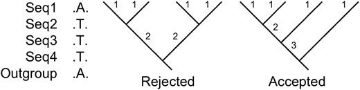
High rejection rate of genealogies when a full mutation frequency spectrum is considered. One mutation (A → T) of size 3 was observed in four sequences. There are two types of rooted topologies for four sequences. Of the two types, only the second one can explain the data because it has a branch of size 3. Therefore, 33.3% (Tajima 1983) of the simulated random genealogies are inconsistent with the observed data.
Using the compact mutation frequency spectrum, however, allows us to sample genealogies effectively. The probability is 1 that a genealogy has at least one internal branch with size ≥3 when n ≥ 5. Then, a uniform sampling strategy can be used, and each random genealogy is consistent with the data. This sampling strategy is different from both importance sampling (Griffiths and Tavaré 1994) and the Markov chain Monte Carlo method (Kuhner et al. 1995).
Since it is impossible to obtain an analytical expression for the likelihood function, a simulation approach is proposed. Equation 2 requires a summation over a huge number of topologies, and each topology has an infinite number of possible branch lengths. Therefore, rather than sampling all genealogies, we consider a large random sample of G. The approach is possible and efficient because each simulated G is consistent with the compact mutation frequency spectrum over m loci (D) when
Simulate genealogies (topology without mutation) for m loci conditioned on the position of selected site (M),
\(\mathrm{{\hat{{\alpha}}}}\)and\(\mathrm{{\hat{{\tau}}}}\).- Compute the value of\(L_{\mathbf{\mathrm{G}}}\)aswhere\[L_{\mathbf{\mathrm{G}}}{=}P(\mathbf{\mathrm{D}}{\vert}\mathbf{\mathrm{G}}){=}{{\prod}_{k{=}1}^{m}}P(\mathrm{{\xi}}_{1k}{\vert}G_{k})P(\mathrm{{\xi}}_{2k}{\vert}G_{k})P(\mathrm{{\xi}}_{Xk}{\vert}G_{k}),\]\(P(\mathrm{{\xi}}_{i}{\vert}G)\)is given by the Poisson probability,with\[P(\mathrm{{\xi}}_{i}{\vert}G){=}\frac{\mathrm{{\lambda}}^{\mathrm{{\xi}}_{i}}e^{{-}\mathrm{{\lambda}}}}{\mathrm{{\xi}}_{i}!},\]\(\mathrm{{\lambda}}{=}l_{i}\mathrm{{\theta}}/2\)and\(l_{i}\)as the length of the branches with size i, and\(l_{X}{=}{\sum}_{i{=}3}^{n{-}1}l_{i}\). The length of the branches is scaled such that 1 unit represents 2N generations.
Repeat steps 1 and 2 K times. Then
\({\hat{L}}{=}(1/K){\times}{\sum}_{\mathbf{\mathrm{G}}}L_{\mathbf{\mathrm{G}}}\).
Obviously, the accuracy of the estimation is improved by using large values of K. In the following, this procedure is denoted by L1. In addition, we propose a similar procedure, L2, as follows. The K simulations conditioned on M, given
The composite-likelihood method of Kim and Stephan (2002) (henceforth called KS) can be compared with L1 and L2. However, a minor revision is needed because the KS method is designed for continuous sequences under the infinite-site model. In this study, it is assumed that a locus in the KS model is composed of 300 nucleotide sites, and each nucleotide site within the locus has the same recombinational distance to the selected site, and there is no recombination within the loci.
The likelihood-ratio test (LRT) is a statistical test of the goodness-of-fit between two models. Neutrality can be seen as a special case of hitchhiking, namely that the selected site is far away from the considered region such that there is no hitchhiking effect observed within the region. Hence,
RESULTS
The parameters α or τ can be estimated by the methods of Kim and Stephan (2002) and Przeworski (2003) or simply assigned by the following procedure. For a fixed value of the recombination rate, the length of the chromosomal region affected by a single hitchhiking event depends primarily on the strength of selection (Figure 2). A large region is affected when selection is strong, and thus the assigned strength of selection
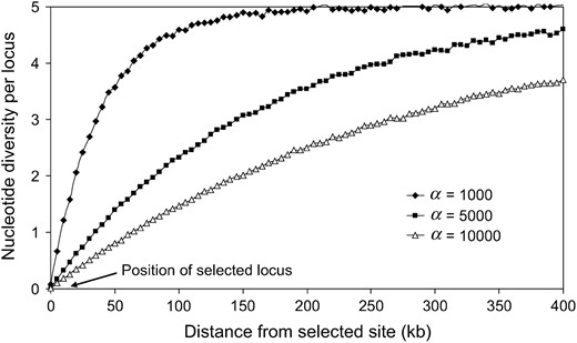
The effect of positive selection with different strength. The average level of nucleotide variation is plotted as a function of the distance (in kilobases) from the selected site. N = 100,000 and n = 10.
![Illustration of the log-likelihood curve for one simulated data set with a positive selection event occurring at 100 kb. The estimated position of the selected site is at 105 kb. N = 100,000, n = 10, m = 10, θk = 5, K = 1000, $\batchmode \documentclass[fleqn,10pt,legalpaper]{article} \usepackage{amssymb} \usepackage{amsfonts} \usepackage{amsmath} \pagestyle{empty} \begin{document} \(\mathrm{{\hat{{\alpha}}}}{=}\mathrm{{\alpha}}{=}1000\) \end{document}$, and $\batchmode \documentclass[fleqn,10pt,legalpaper]{article} \usepackage{amssymb} \usepackage{amsfonts} \usepackage{amsmath} \pagestyle{empty} \begin{document} \(\mathrm{{\hat{{\tau}}}}{=}\mathrm{{\tau}}{=}0\) \end{document}$. The positions of the neutral loci are shown at the bottom.](https://oup.silverchair-cdn.com/oup/backfile/Content_public/Journal/genetics/171/1/10.1534_genetics.105.041368/3/m_41368f3.jpeg?Expires=1716884549&Signature=bcdo-Iphm0VlWfIc9MIRe7RLHfBMobjEIwwLn2IyFqtJkMxJggUPbkqPgmNeOYjcBMvUzAOTurlTFYnQz8~EcQD8uZ8P0~Gd7409tRDSctfpCFSDEspCMwEfdTdGXCl2ewvkgGfwiiR~RysfPlRqjezYi4iUMPgbLCCrHILdnuFPghqZ8XEx4dmSs9NPs8G8vU58TRhQ1V6bXMqjb7Ar6cgKZuXZY2mCjWBxURzdNfzDuTrB8MGf~6~5vAmhC0Imtf6Rw4RO6lhYT5X~-EW4yIDjNeACioZUaDWvuANuvKCyHqCexPpGDhIHInXPtNeaCZ2zJadzXegNk1wlSjypsg__&Key-Pair-Id=APKAIE5G5CRDK6RD3PGA)
Illustration of the log-likelihood curve for one simulated data set with a positive selection event occurring at 100 kb. The estimated position of the selected site is at 105 kb. N = 100,000, n = 10, m = 10, θk = 5, K = 1000,
Let us consider a certain region and assume that selection occurred at the center of the region. Then, what is the standard deviation of estimated position of the selected site given randomly selected samples and loci? The standard deviation of the estimated target position of selection is given in Table 1 and Figure 4 when α and τ are known (namely,
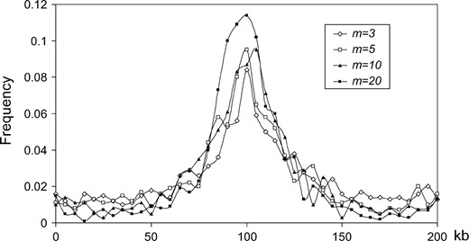
The distribution of the estimated position of selection (from 1000 simulated data sets). Parameter values are the same as in Figure 3, and the positions of the m neutral loci in 1000 simulated data sets have been chosen according to method LPS1.
The standard deviation (SD) of the estimated position of the selected locus, the power of the tests, and the false positive rates
SD (kb) | Power (%) | False positives (%) | |||||
|---|---|---|---|---|---|---|---|
| m | KS | L1 | L2 | L1 | L2 | L1 | L2 |
| 3 | 42.0 | 43.0 | 44.0 | 72.8 | 87.6 | 20.0 | 36.8 |
| 5 | 37.8 | 38.4 | 36.3 | 93.6 | 93.4 | 41.4 | 38.7 |
| 10 | 31.0 | 33.8 | 29.8 | 96.7 | 97.4 | 26.9 | 28.0 |
| 20 | 23.0 | 28.7 | 20.2 | 93.0 | 97.6 | 7.8 | 11.4 |
The parameter values are n = 10,
If the selected site lies at the center of the region, the estimated position of the selected site is always unbiased even if the distribution of the estimated position is uniform. Therefore, we also considered the cases that the target of selection is located at the edge of the region (Table 2). Generally, L1 and L2 are less biased than the KS method, and the more neutral marker loci are surveyed, the less biased the estimation becomes. Moreover, when the selected site lies at the edge of the region rather than at the center of the region (Table 1), standard deviation is larger and the power smaller.
The standard deviation (SD) of the estimated position of the selected locus, the power of the tests, and the false positive rates
Average estimated position (kb) | SD (kb) | Power (%) | False positives (%) | |||||||
|---|---|---|---|---|---|---|---|---|---|---|
| m | KS | L1 | L2 | KS | L1 | L2 | L1 | L2 | L1 | L2 |
| 3 | 66.8 | 58.9 | 61.0 | 62.6 | 60.3 | 63.4 | 52.3 | 68.8 | 21.8 | 39.9 |
| 5 | 57.3 | 49.9 | 47.8 | 57.5 | 55.9 | 58.9 | 80.4 | 81.8 | 42.5 | 37.9 |
| 10 | 45.1 | 33.7 | 29.0 | 50.4 | 49.8 | 47.6 | 84.8 | 85.9 | 28.2 | 25.6 |
| 20 | 34.6 | 18.3 | 19.6 | 43.6 | 34.4 | 36.6 | 77.2 | 89.9 | 6.4 | 8.9 |
The parameter values are the same as in Table 1, and the selected site is at the left edge of the region.
Usually the strength of selection and the time of the hitchhiking event in the past are unknown. Table 3 gives the effect of the difference between the assigned or estimated parameter values (
The effect of the difference between assigned (
α = 1,000 | α = 2,500 | α = 5,000 | α = 7,500 | α = 10,000 | |
|---|---|---|---|---|---|
| Standard deviation of estimated position of selected locus (kb) | |||||
| τ = 0 | 115.5 | 76.1 | 57.8 | 60.5 | 60.4 |
| τ = 0.01 | 120.1 | 74.2 | 63.3 | 64.5 | 64.8 |
| τ = 0.02 | 120.6 | 76.5 | 57.3 | 59.8 | 62.7 |
| τ = 0.05 | 129.9 | 88.5 | 69.7 | 70.5 | 72.0 |
| τ = 0.1 | 143.5 | 103.9 | 86.6 | 82.7 | 83.2 |
| τ = 0.15 | 149.2 | 119.8 | 103.3 | 100.4 | 100.6 |
| τ = 0.2 | 156.4 | 132.5 | 119.3 | 115.8 | 115.0 |
| τ = 0.5 | 175.8 | 165.8 | 164.3 | 162.6 | 161.9 |
| Power (%) | |||||
| τ = 0 | 18.9 | 74.8 | 96.0 | 98.6 | 99.3 |
| τ = 0.01 | 17.4 | 74.0 | 96.3 | 99.5 | 99.9 |
| τ = 0.02 | 15.9 | 73.0 | 97.0 | 99.5 | 99.9 |
| τ = 0.05 | 12.1 | 64.5 | 92.7 | 98.4 | 99.4 |
| τ = 0.1 | 4.9 | 41.2 | 82.4 | 93.4 | 98.7 |
| τ = 0.15 | 4.2 | 28.4 | 66.2 | 83.6 | 89.9 |
| τ = 0.2 | 2.1 | 18.3 | 48.5 | 67.6 | 74.8 |
| τ = 0.5 | 0.4 | 1.7 | 5.0 | 6.7 | 8.9 |
The effect is measured by the power of the test (with
This suggests that a minimum strength of selection is detectable given the data. A large number of loci is required to obtain a low false positive rate, for example, 5%, and thus the size of the region cannot be reduced indefinitely. Therefore,
Next we consider different ways to choose the neutral loci (Figure 5). The LPS2 method generates less standard deviation than LPS1 in all comparisons. This is because the positions of neutral loci chosen according to LPS2 are more likely to be equally distributed than those of LPS1, and thus the former contains more information on the spatial distribution of polymorphisms. Thus, to increase the chance of detecting the hitchhiking event, it is recommended that, if possible, the marker loci should be equally or nearly equally distributed along the chromosome or within candidate regions.
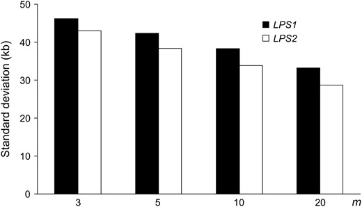
Standard deviation of the estimated position of the selected site for LPS1 and LPS2 and different numbers of loci. Parameter values are the same as in Figure 3.
In practice, the sequencing load is often a limiting factor. The more loci are chosen, the less base pairs per locus can be sequenced, and vice versa. Figure 6 displays the effect of the different choices. All comparisons show clearly that the first strategy (solid box) is better than the second one (open box). Therefore, we recommend that the priority should be put on the number of loci. By increasing the sequenced length per locus, more segregating sites are expected, so a more precise estimation of the level of local polymorphism can be obtained. However, Figure 6 shows that obtaining more information on the spatial distribution of polymorphisms along the whole region is more important than getting more precise estimates of local levels of polymorphism.
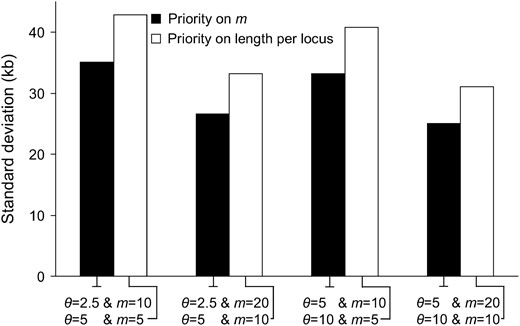
Standard deviation of the estimated position of the selected site for different sequencing strategies (m vs. length of marker locus). The solid bars represent the cases with more loci and a shorter sequence per locus. The open bars represent the alternative strategy (such that the sequencing load in both cases is identical). Parameter values are the same as in Figure 3. LPS2 is used.
Finally, we consider the case that the priority is given to the number of sampled chromosomes (n) rather than to the number of loci (m) (Figure 7). The priority given to the number of loci is the better strategy when the number of loci is not very large. This difference disappears when the number of loci gets large.
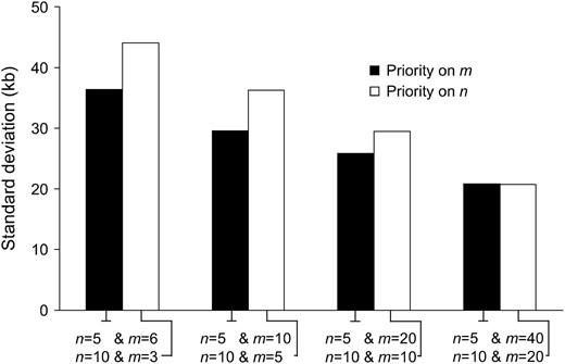
Standard deviation of the estimated position of the selected site for different sequencing strategies (m vs. n). The solid bars represent the cases with fewer sampled chromosomes and more loci and the open bars the cases with more sampled chromosomes and fewer loci. Parameter values are the same as in Figure 3. LPS2 is used.
APPLICATION
The proposed likelihood methods were applied to a region on the X chromosome of D. melanogaster. The analyzed region extends over 660 kb. The region was selected due to the dense distribution of marker loci. This region contains 19 fragments that are nearly uniformly distributed over the region (Figure 8). The data for seven of these loci are from Glinka et al. (2003); the remaining data were kindly supplied by Lino Ometto and Sascha Glinka. On the basis of the published data (Glinka et al. 2003), the mean of θ across the X chromosome in the European and African populations is 0.0044 and 0.0127 per site, respectively, so that the value of θ for each fragment is obtained as the mean value per site times the length of the fragment (excluding insertions and deletions). The estimated recombination rate is 3.8 cM/Mb (Glinka et al. 2003). The ancestral status of each polymorphic nucleotide site was determined by comparison with the D. simulans sequence (Glinka et al. 2003).
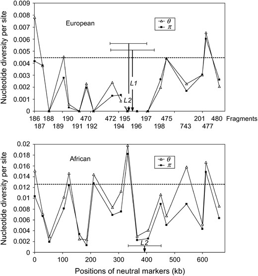
Genetic diversity of Drosophila melanogaster between African and European populations. The dashed lines are the expected θ-values for each population. (Top) Fragments are denoted according to their identification numbers (Glinka et al. 2003). (Bottom) Their positions on the X chromosome are shown. The positions of selected sites estimated by L1 and L2 and their 95% confidence intervals are also presented. For the African population, only the L2 method suggests the occurrence of a sweep.
To perform our analyses, the selection coefficient (ŝ) we assigned was 0.053, so that h, the relative heterozygosity, was 0.92 at the edge of the region. Moreover, we used
In the European population, the likelihood-ratio test via L1 and L2 rejected the standard neutral model in favor of the selective sweep model at the 5% level. It suggests that the observed polymorphism in the 19 partially linked fragments can be explained better by the hitchhiking model with the assigned ŝ- and
In the European population, the positions of selected site estimated by L1 and L2 differ slightly. Both of them are between fragments 195 and 196 (the positions are 18.5 and 5.1 kb away from fragment 195, respectively). The 95% confidence regions of the positions estimated by L1 and L2 are shown in Figure 8. The 10,000 simulated data sets also show that the power of the tests is 96.3 and 97.5%, and the false positive rate is 11.3 and 15.7% for L1 and L2, respectively.
In the African population, the position of the selected site estimated by L2 is between fragments 196 and 197 (14.3 kb away from fragment 197), which is rather close to the positions estimated by L1 and L2 in the European population. The simulated data sets also show that the power of the test is high (97.7%) and the false positive rate low (7.9%) for L2. The 95% confidence region of the position estimated by L2 is shown in Figure 8. It overlaps with those of the European population.
DISCUSSION
Method:
In this study, two exact-likelihood methods are proposed. The methods are generally based on coalescent simulations using the ancestral recombination graph. Furthermore, the compact mutation frequency spectrum is used to compute the likelihood.
In the proposed methods, L2 shows a lower standard deviation in the estimated position of selection than L1 in some cases because of the difference in dealing with branch lengths. There is a large variance of branch length in individual simulations in L1, while in L2 the variance is reduced by averaging the branch lengths. Furthermore, to understand this difference, let us consider the genealogies under hitchhiking for two loci with two sampled chromosomes. In some cases, there is no recombination between the two loci, so that the two branches will coalesce. And thus the distance between loci is not counted efficiently by the likelihood in L1. However, by averaging the branch length among simulations, a shorter average branch length will be observed in the locus that is closer to the selected site, and thus the distance between loci is counted by the likelihood in L2.
However, L1 also shows a lower standard deviation of the estimated position of selection than L2 in some cases. This is because information on correlations among loci is discarded in L2. Thus, both L1 and L2 are recommended in practice. For a given genomic region, the estimated positions of the selected site by L1 and L2 could be different. In such a case, the variance of estimated position of the selected site can be obtained, and the method generating a lower variance should be used.
Unlike the Bayesian approach (Przeworski 2003), the proposed likelihood methods do not incorporate prior information about the model parameters. If we expect that beneficial mutations occur preferentially in coding and control regions, the Bayesian approach may be helpful.
A global sweep in D. melanogaster:
In application, the two proposed methods were applied to 19 partially linked loci on the X chromosome of D. melanogaster. The hitchhiking model was accepted for the assigned parameters, and the position of the selected site (estimated by the various methods) falls into a 54-kb region. The divergence between D. melanogaster and D. simulans in this region is at the same level as the average divergence between the two species over the whole X chromosome (data not presented). Thus the deficiency of polymorphism cannot be explained by a relatively low mutation rate. Given the fact that the hitchhiking model was accepted in both the European and African populations, we suggest that a recent hitchhiking event may have occurred in the ancient African population. As the confidence intervals of the estimated positions overlap in the African and European populations, this selective sweep may have continued in the European population driven by the same selected allele. The sweep in Africa is likely to be older as levels of nucleotide diversity are higher than those in Europe. Thus we may have a global selected sweep. Alternatively, two independent local hitchhiking events have to be postulated, one in the European population and another in the African population. These alternatives may be distinguished by mapping the positions of the selected sites more precisely on the basis of more densely spaced marker loci. For the time being, a global sweep is the more parsimonious explanation.
In this study, we did not consider the effect of demography, such as population size bottlenecks and expansions. However, our approach can be extended to analyze populations with variable size. Finally, we note that the methods can also be used to estimate α and τ after minor revision, but it would consume much more computing time.
Footnotes
Communicating editor: D. Rand
Acknowledgement
We thank David De Lorenzo, Sascha Glinka, and Lino Ometto for providing unpublished data and Joachim Hermisson and Sylvain Mousset for helpful discussions. This work was funded by the VolkswagenStiftung (grant I/78815).
References
Braverman, J. M., R. R. Hudson, N. L. Kaplan, C. H. Langley and W. Stephan,
Fay, J. C., and C.-I Wu,
Felsenstein, J.,
Fu, Y.-X., and W.-H. Li,
Glinka, S., L. Ometto, S. Mousset, W. Stephan and D. D. Lorenzo,
Griffiths, R. C., and P. Marjoram,
Griffiths, R. C., and S. Tavaré,
Harr, B., M. Kauer and C. Schöltterer,
Hudson, R. R.,
Kaplan, N. L., R. R. Hudson and C. H. Langley,
Kim, Y., and R. Nielsen,
Kim, Y., and W. Stephan,
Kim, Y., and W. Stephan,
Kuhner, M. K., J. Yamato and J. Felsenstein,
Li, W.-H., and Y.-X. Fu,
Maynard Smith, J., and J. Haigh,
Przeworski, M.,
Sabeti, P. C., D. E. Reich, J. M. Higgins, H. Z. P. Levine, D. J. Richter et al.,
Stephan, W., T. H. E. Wiehe and M. W. Lenz,
Storz, J. F., B. A. Payseur and M. W. Nachman,
Tajima, F.,
Wiuf, C., and J. Hein,
