Abstract
Heritability is a population parameter of importance in evolution, plant and animal breeding, and human medical genetics. It can be estimated using pedigree designs and, more recently, using relationships estimated from markers. We derive the sampling variance of the estimate of heritability for a wide range of experimental designs, assuming that estimation is by maximum likelihood and that the resemblance between relatives is solely due to additive genetic variation. We show that well-known results for balanced designs are special cases of a more general unified framework. For pedigree designs, the sampling variance is inversely proportional to the variance of relationship in the pedigree and it is proportional to 1/N, whereas for population samples it is approximately proportional to 1/N2, where N is the sample size. Variation in relatedness is a key parameter in the quantification of the sampling variance of heritability. Consequently, the sampling variance is high for populations with large recent effective population size (e.g., humans) because this causes low variation in relationship. However, even using human population samples, low sampling variance is possible with high N.
HERITABILITY (h2), the proportion of phenotypic variation that is explained by additive genetic variation, is an important parameter in plant and animal breeding, evolutionary genetics, and human and medical genetics. It is central in quantifying the role of genetics in complex traits, predicting response to selection in natural and artificial breeding programs, and determining the limits of trait or disease prediction using information from relatives or DNA markers. Traditionally, the estimation of heritability is from pedigree data, by modeling the observed resemblance between relatives (Falconer and Mackay 1996; Lynch and Walsh 1998). More recently, genetic variation has been estimated using genetic marker information (Ritland 2000; Thomas 2005; Visscher et al. 2006; Yang et al. 2010; Robinson et al. 2013; Berenos et al. 2014). These designs estimate the genetic variance explained by the markers, which may be less than the additive genetic variance (Yang et al. 2010), but in this article we refer to the parameter estimated as the heritability regardless of whether it is estimated from relationships defined by pedigree or by markers. In general, designs to estimate heritability can be grouped by their use of (i) the expected identity-by-descent (IBD) sharing between relatives, i.e., using pedigree relationships, (ii) marker-based estimated IBD relationships between relatives for known pedigree relationships, and (iii) marker-based estimated genomic relationship matrices for unknown pedigree relationships. For a review of these designs with a particular focus on human populations, see Vinkhuyzen et al. (2013).
Even with large sample sizes, the standard error of heritability estimates is often disappointingly large and it varies greatly between experimental designs. Therefore it is important to calculate the expected standard error before committing resources to collecting the data. Given a particular experimental design and the population value of h2, its sampling variance can be determined using a number of methods. After the data have been collected, the (asymptotic) sampling variance of the estimate can be derived from the analysis, for example, from mean squares in balanced designs, from the information matrix when using maximum likelihood or from the posterior density in Bayesian analysis. Prior to collecting data on phenotypes, the sampling variance can be predicted using statistical theory, typically for balanced designs, or obtained from computer simulation for more complex pedigree structures. In this study, we provide a single framework for calculating the asymptotic sampling variance of the heritability across a wide range of designs, for a class of models with two random variables and when analysis is by maximum likelihood (ML). We derive the sampling variance using the expected value of the information matrix. We show that previous results are special cases of the general framework and that the variance in relationships in the sample is a key parameter in all experimental designs.
Model and Assumptions
We assume a linear model with no fixed effects (or fixed effects that have been adjusted for without error) and two random components, a genetic effect (
g), and a residual effect (
e). There are
N individuals, each with a single observation,
y,
where
y,
g, and
e are vectors of length
N of the phenotypic observations, genetic value, and residuals, respectively.
G is the genetic relationship matrix (GRM), either from pedigree relationships, in which case it is the usual numerator relationship matrix (twice the kinship matrix), or derived from SNP similarity (
Vanraden 2008;
Stranden and Garrick 2009;
Yang et al. 2010). The genetic, residual, and total variances are
σg2,
σe2, and
σ2, respectively. The
N ×
N covariance matrix of all observations (
V) is
where
h2 =
σg2/(
σg2 +
σe2) =
σg2/
σ2, the heritability.
General Formula for Sampling Variance
We can decompose the symmetric GRM as
with
TT′ =
T′
T =
I and
T−1 =
T′ because
T is orthogonal and
D a diagonal matrix containing eigenvalues (
λi) of
G. Inference on
h2 from data
y does not change upon a linear transformation of
y. We can therefore transform
y by using the eigenvectors of
G, which for the simple model used here are also eigenvectors of
V (
Thompson and Shaw 1990,
1992;
Lippert et al. 2011;
Blangero et al. 2013;
Raffa and Thompson 2014).
with
The log likelihood with respect to
h2 and
σ2 is
as shown previously (
Thompson and Shaw 1990;
Raffa and Thompson 2014). Equation 1 is very similar to that in
Blangero et al. (2013), but with added parameter
σ2. Elements of the (Fisher) information matrix (
F) are obtained by taking the second derivative of (1) taken at the maximum with respect to
h2 and
σ2, and then the negative value of its expectation over
y*, using
The derivation of the first element of
F (
F11) is given here. The other two elements are derived analogously,
and so
The resulting elements of the 2 × 2 matrix
F are
with constants
a and
b,
and
These elements are similar to those presented in
Thompson and Atkins (1994), who parameterized the likelihood in a genetic and residual variance component, whereas we have parameterized in heritability and phenotypic variance. Thompson and Atkins do not have the factor
and have λ
i2 and λ
i in the equations above where we have (
λi – 1)
2 and (
λi – 1), respectively, the difference due to the choice of parameters in the model. In the article that developed the method of estimation of variance component in linear mixed models using restricted maximum likelihood (
Patterson and Thompson 1971), the authors presented both the log likelihood and the information matrix in terms of eigenvalues of the covariance matrix.
The asymptotic sampling (co)variance for the estimates of heritability and phenotypic variance are from
F−1. Therefore, the asymptotic sampling variance of the estimate of the heritability is
Hence, under the assumptions given, this is a completely general expression for the asymptotic sampling variance of an estimate of heritability and depends only on the eigenvalues of the GRM, the population value of heritability, and the experimental sample size.
Special Cases
With additional assumptions or for balanced designs, terms for a and b simplify and simple solutions for the sampling variance of can be derived. We go through a number of these special cases in this section that encompass pedigree and marker-based GRM.
Phenotypic variance (σ2) known
In many applications, the sampling variance of the total phenotypic variance is small or known before the experiment is conducted, and therefore it is useful to consider the sampling variance of heritability under the assumption that the phenotypic variance is known without error. For example,
Blangero et al. (2013) assume that
σ2 is known in their derivations of the expected likelihood-ratio-test statistic (ELRT). If we assume here that the phenotypic variance is known without error then the resulting sampling variance of the estimate of heritability is
This expression is smaller than that in (2); hence assuming that phenotypic variance is known when it is not will lead to an underestimate of the sampling variance of heritability. This underestimate will be small when
b2/
N is small relative to the term
a.
For a small heritability,
a →
b →
and
Assuming that the phenotypic variance is known and
h2 is small gives
which is close to (4) because the mean eigenvalue will be 1 in the absence of inbreeding when the GRM is from pedigree identity-by-descent and very close to 1 when the GRM is estimated from SNP data (
Janss et al. 2012). Hence, when the population value of heritability is small, its sampling variance is only a function of the variation in relatedness and sample size.
All
Equation 4 is also the result for when all λi are close to 1, such that their variance approaches zero. This situation can occur when the GRM is created from population SNP data on unrelated individuals in a population with a large effective population size. However, as we derive below, the variance of eigenvalues depends both on experimental sample size and effective population size, and so these parameters affect the sampling variance of heritability. In particular, the variance in eigenvalues is proportional to experimental sample size, so the larger the sample size the wider the spread around a mean value of 1.
Pairs of relatives with relationship r
If there are
m pairs of relatives of the same degree
r, then 2
m =
N and there are
m eigenvalues
λ1 with value 1 +
r and
m eigenvalue λ
2 with value 1 −
r (
Searle 1982;
Blangero et al. 2013). Let
ρ =
rh2. Then
and
For pairs of monozygotic (MZ) twins (
r = 1), Equation 5 becomes var(
) = (1 –
ρ2)
2/
m. For pairs of full-sibs (
r =
), the sampling variance is 4(1 –
ρ2)
2/
m. For bivariate normality, the sampling variance of a correlation coefficient between two variates with population value
ρ is ∼(1 –
ρ2)
2/
N (
e.g.,
Lynch and Walsh 1998, p. 819), so consistent with Equation 5.
Balanced design of multiple families
For
m families with
n individuals of relationship
r, there are (
n − 1) eigenvalues of (1 –
r) and 1 eigenvalue of (1 +
r(
n – 1)) per family. This follows from known results on eigenvalues for symmetrical matrices that can be written as
cI +
dJ, with
c and
d constants (
Searle 1982). Substituting these eigenvalues into the equation for parameters
a and
b gives
and
This is consistent with the intraclass correlation sampling variance (
e.g.,
Falconer and Mackay 1996, p. 180), apart from having
m in the denominator [the least-squares derivation has (
m − 1) instead]. Although we have assumed no fixed effects, in practice at least a mean would be included in the model and this absorbs one degree of freedom from the comparison of families. The least-squares formula takes account of this but ML estimation ignores it. Assuming that the phenotypic variance is known gives
smaller than (5) by a factor of 1/(1 + ρ
2(
n − 1)). For large half-sib families, this term can be substantial.
Twin design
In human populations, the classical twin design is common for estimating genetic and nongenetic variance components. Let
N = 2
mM + 2m
D, with
mM and
mD the number of MZ and dizygotic (DZ) pairs, respectively. In total, there are four different eigenvalues: 2, 0, 3/2, and 1/2 (
Blangero et al. 2013), with multiplicity
mM,
mM,
mD, and
mD. Let
c =
mM/(
mM +
mD), the proportion of all twin pairs that are MZ pairs. Using Equation 5,
a −
b2/
N =
NT, with
and
This analysis assumes that there are no common environmental effects so the sampling variance is not appropriate for the usual practice of estimation of heritability using maximum likelihood fitting both an additive genetic and common environmental component (
Neale and Cardon 1992).
Within-family estimation using realized relationships estimates from markers
Full-sibs have an expected pedigree relationship of 0.5 but the actual amount of the genome shared varies around 0.5 and this realized relationship can be estimated using genetic markers and used to estimate heritability (
Visscher et al. 2006,
2007;
Hemani et al. 2013). These relationships can be estimated using identity-by-descent calculations conditional on observed marker genotypes. For full-sibs and half-sibs in human populations, the standard deviation of realized relationships is ∼0.04 and 0.03, around the expected value of
and
, respectively. For a comprehensive theory on the variance of realized relationships, see
Hill and Weir (2011). A feature of this design is that common environmental factors that vary between families do not bias the heritability estimate.
Visscher et al. (2006) derived an approximate sampling variance of the estimate of heritability from multiple families with two full-sibs each.
Hill (2013) derived the sampling variance of the estimate of genetic variation using REML for the general case of
f families each of size
n and expected relationship
θ (twice the kinship coefficient). We can use the same general framework as developed here to approximate the sampling variance from within-family estimation. The difference between this design and those previously discussed is that the GRM is not fixed. That is, the eigenvalues of the GRM are themselves random variables and to derive the sampling variance of the estimate of heritability we need to first derive the expected value of the elements of the Information matrix over repeated samples. We provide details of an approximation in
Appendix A. It results in
This equation shows that the sampling variance reduces by the square of the sample size per family (
n), essentially because every individual adds a contrast with all other family members in the sample. As detailed in
Appendix A, this approximation breaks down when
h2 and
n are large.
Random sampling from the population
One design to estimate the amount of additive genetic variation captured by SNPs is to take a random sample of individuals from the population, derive a GRM from SNP similarity, and estimate variance components from (residual) maximum likelihood (
Yang et al. 2010). In this sampling scheme, individuals are not sampled or ascertained based upon particular pedigree relationships, and any pedigree relationship, if known, is not taken into account in the analysis. The sampled individuals are related to some extent, even if very distantly, because the population size is finite. In human populations, this sampling scheme corresponds to sampling individuals who are conventionally unrelated. As for the case of realized relationships within families, the GRM is not fixed. We approximate
E(
a) and
E(
b2) in
Appendix B. The resulting sampling variance of the estimate of heritability is
where
v(
θ) is the variance of relatedness in the population, which is a function of effective population size (
Goddard 2009;
Goddard et al. 2011). Analogous to the within-family design, the sampling variance is inversely proportional to the square of the sample size, rather than by 1/
N in pedigree designs.
Rijsdijk and Sham (2002) derived the same result (parameterized as the noncentrality-parameter, NCP, of the test statistic for heritability) for QTL linkage mapping in pedigrees, assuming that the variance in relatedness is small. Equation 8 was previously derived for SNP-based estimation of variance components from linear regression theory, assuming that the phenotypic variance is known without error (
Vinkhuyzen et al. 2013;
Visscher et al. 2014).
Statistical Power
The interest in this study is not about hypothesis testing but about quantifying the sampling variance of the estimate of heritability. For a detailed treatment on statistical power in variance component estimation using (restricted) maximum likelihood we refer to previous publications (Self and Liang 1987; Shaw 1987; Thompson and Shaw 1990; Almasy and Blangero 1998; Williams and Blangero 1999; Rijsdijk et al. 2001; Purcell et al. 2003; Raffa and Thompson 2014). Here we briefly consider the expected value of two test statistics that have been used for hypothesis testing in variance component estimation, the Wald test, and the likelihood-ratio-test statistic.
The Wald test is based on
/var(
), which under the null hypothesis that
h2 = 0, follows a χ
2 distribution. However, if
h2 > 0, the Wald test statistic follows approximately a noncentral χ
2 with noncentrality parameter (NCP
W)
If the estimation of phenotypic variance is ignored, then
Alternatively, the null hypothesis that
h2 = 0 can be tested with a likelihood-ratio test. Blangero and colleagues (
Blangero et al. 2013) presented a very simple equation for the ELRT statistic to test the null hypothesis of
h2 = 0,
Equation 11 converges to Equation 10 when
h2(λ
i − 1) → 0. For pairs of relatives with relationship
r, NCP
W =
Nr2h4 / (1 –
r2h4) and NCP
LRT = −
N ln(1 −
r2h4). These expressions are equivalent when
r2h4 → 0. When the true parameter is far from the one being tested under the null, these expressions can give quite different values.
Raffa and Thompson (2014) give an analysis based on asymmetrical confidence intervals for the heritability.
Numerical Examples
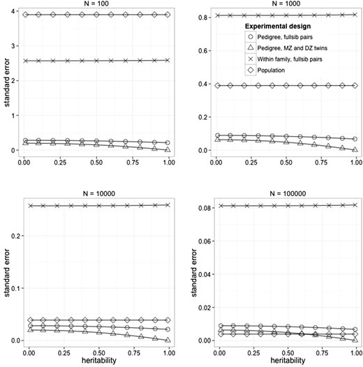
Figure 1 shows the approximation to the standard error of an estimate of heritability as a function of the population value, experimental sample size, and design. Four different designs were used: a pedigree design of unrelated full-sib pairs, a pedigree design with MZ and DZ twins pairs with a ratio of 1:2 MZ and DZ pairs, a within-family design using full-sib pairs, and a population design using nominally unrelated individuals. In the last two designs, GRM are estimated with SNP data. These designs are less powerful than the pedigree-based experimental designs, but make fewer assumptions. At N = 10,000 the sampling variance of the population design approaches that of the pedigree designs, and at N = 100,000 it becomes the most powerful design. Sample sizes of 100,000 are realistic in human population and even larger samples sizes are expected in the next few years. Therefore, strong inference on heritability can be drawn using random samples from the population, while not having to make assumptions about the resemblance between relatives due to common environmental factors. The within-family design, which is the most robust with respect to assumptions of the model, remains inaccurate even when the analysis is on 50,000 full-sib pairs. However, in species such as fish with huge full-sib family sizes, accurate estimation could be achieved (Odegard and Meuwissen 2012; Hill 2013).
Figure 1
Standard error of estimates of heritability from different experimental designs in human populations, as a function of the population value of the heritability (x-axis), experimental sample size, and experimental design. For the within-family design (Within-family estimation using realized relationships estimates from markers), the variance in realized relationships was assumed to be 0.0392. For the population design (Random sampling from the population), the variance is relatedness was approximated assuming Ne = 10,000, a genome length of 35 M, and an average chromosome length of 1 M (Goddard 2009).
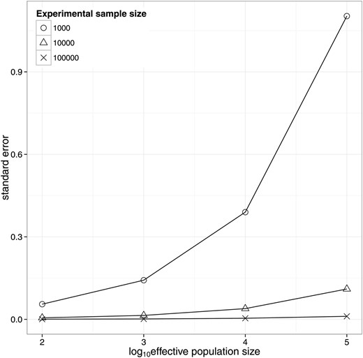
Figure 2 shows results for the population design for species with different Ne values of 1000, 10,000, and 100,000. It shows the increase in sampling variation with increasing effective population size, which is due to the decrease in the variation in relatedness. For the within-family design the sampling variance of heritability does not depend on the effective population size.
Figure 2
Standard error of the estimate of heritability from random samples of individuals from populations with different effective size and SNP-derived relationship matrices. For each population, a genome length of 35 M and an average chromosome length of 1 M was assumed (Goddard 2009).
Discussion
We have presented a general framework to quantify the sampling variance of heritability as a function of its population value, the sample size (N), and experimental design. Figure 1 shows that the sampling variance is relatively insensitive to the true value of h2 except when h2 → 1. The results recapitulate results from balanced designs and show that for pedigree designs, the sampling variance tends to be proportional to 1/N. In contrast, for designs that use genetic markers to estimate relatedness within families or estimate relatedness among randomly sampled individuals, the sampling variance is proportional to 1/N2. Consequently, very large samples of “unrelated” individuals are powerful for estimating h2. The key feature of the experimental design is the variation in relatedness. This is small within families of full-sibs and consequently the sampling variance of h2 is large.
There are a number of limitations to our study. First, we have assumed that the parameter whose sampling variance we derive is the same in different experimental designs. Even in the absence of confounding factors such as common environmental effect or nonadditive genetic factors, this is not necessarily the case. For the pedigree and within-family design, the parameter given our model assumptions is the narrow-sense heritability. But for the population design it is the proportion of phenotypic variance captured by genetic markers. If these markers are not sufficiently correlated with the genetic variants that cumulatively contribute to the total narrow sense heritability, then the use of a marker-based GRM will estimate additive genetic variation that is less than the total additive genetic variance. This can occur if the properties of the markers used to create the GRM are different from the segregating causal variants, for example, if the GRM is based upon common SNPs and the causal variants have lower heterozygosity, leading to loss of information due to imperfect linkage disequilibrium (Yang et al. 2010). Although a “marker heritability” is conditional on the markers used to estimate relatedness, it is a valid population parameter with predictable sampling properties (as shown in this study). In human populations, it has been used to address the question of “missing heritability” from genome-wide association studies (Yang et al. 2010).
Second, we assume that all resemblance between relatives is due to additive genetic covariance, so that there are only two random effects in the model. Additional random effects, for example, common environmental effects, make the covariance matrix V more complicated and generally not diagonalizable. When there are additional variance components, the residual variance as used in this study is partitioned in two or more components. These additional components are also estimated with error and will have a sampling covariance with the estimate of heritability. We suspect that having additional variance components in the model will tend to increase the sampling variance of the heritability, except for some balanced designs. However, we have not investigated general properties for designs with multiple random effects. With more than two variance components, computer simulation might be an efficient way to quantify the sampling variance of heritability and the proportion of variance due to additional random effects.
A third assumption is that estimation is by maximum likelihood or, alternatively, that fixed effects and covariates have been adjusted for without error. In practice, researchers tend to use least squares for balanced designs and restricted maximum likelihood (REML) or Bayesian methods for unbalanced designs. The difference in sampling variance between ML and REML is small when there are few fixed effects relative to the sample size, as, for example, in human genetic applications, but larger in situations where there are many fixed effects (e.g., in livestock applications).
Recently, Raffa and Thompson (2014) extended the work of Blangero et al. (2013) by deriving approximations to the ELRT and confidence intervals of the heritability estimate using Taylor series expansions of the expected likelihood-ratio test with respect to the distribution of the eigenvalues of a given pedigree. Their simplest approximation can be expressed as an approximate sampling variance of the estimate of heritability as 2/[(N − 1)var(λ)] ≈ 2/(N var(λ)). This expression is the same as our special cases and All. The authors show that this approximation is not accurate when the assumptions break down, in particular when eigenvalues are not closely distributed around the mean of 1, and provide a better approximation using the logarithm of the eigenvalues (Raffa and Thompson 2014). They also show that confidence intervals of the estimates of heritability are not symmetrical when the variance in eigenvalues is large and that Wald statistic-based confidence intervals can be too narrow, implying that the use of the derived standard errors in our study to construct a confidence interval can be anticonservative. Although the derivations from Raffa and Thompson were for a pedigree design, they should also apply to other experimental designs, such as those where GRMs are estimated from marker data.
In conclusion, we have proposed a general unified framework to assess the sampling variance of the estimate of heritability using pedigree or marker-based relationships and have quantified how the sampling variance depends on sample size and the variation in relatedness.
Acknowledgments
This study was inspired by John Blangero’s presentation at the 2013 Statistical and Quantitative Genetics conference in Seattle. We thank Bill Hill for discussions and helpful comments, Jesse Raffa for useful comments, and Matt Robinson and Kostya Shakhbazov for feedback and help with R. This research was supported by U.S. National Institutes of Health (NIH) grant R01 GM075091.
Appendix A: Derivation of the Sampling Variance of Heritability from Within-Family Designs
As before, y = g + e, with var(g) = Gσg2 and var(e) = Iσe2. If all individuals belong to a family, E(G) = I on diagonals and θ on off-diagonals. We extract the family mean (u) from an individual’s breeding value so y = u + g* + e, where var(g*) = (G − θJ)σg2 = Wσg2. If we treat u as fixed, then var(y − u) = Wσg2 + Iσe2. The mean eigenvalue of W is (1 − θ) and the variance of eigenvalues is n × var(rij) where rij is the realized relationship between individuals i and j within the same family.
As in
Hill(2013), we derive the sampling variance for a single family of size
n. Under our assumed model of no environmental effects shared by family members,
t =
θh2. As before, the elements of the information matrix are
F11 = 1/2a,
F12 =
F21 =
b/
σ2,
F22 =
n/
σ4. We approximate the elements of the information matrix by taking a second-order Taylor series about the mean eigenvalue of (1 −
θ). Then, approximately,
Using these to construct the (
F−1)
1,1 gives
Using this approximation, the determinant of the information matrix, and therefore the approximation of the sampling variance of heritability, can be negative, when
n > (1 −
t)
2/(
h4 × var(
rij)). For example, for full-sibs (var(
rij) ∼0.038
2) and
h2 = 0.8 (and
t = 0.4), a sampling size of
n = 390 full-sibs would result in a predicted sampling variance of the estimate of heritability that is negative. Presumably a higher-order Taylor series would correct this, but at the expense of having a relatively simple expression.
If we now use the eigenvalue decomposition of
W, as in Thompson and Atkins (1994) and as used in our other designs but parameterizing the variance components instead of
h2 and
σ2, then the element of the Information matrix (
S in the Hill notation) are
If we take expectations of
a,
b, and
c, where the expectation is over the eigenvalues of
W [with mean = (1 −
θ), variance = var(λ)
n × var(
rij)], then, from a second-order Taylor series about the mean:
Finally, the sampling variance of the estimate of
σg2 is, approximately,
These terms are similar but not identical to
Hill(2013). The difference is because we use ML whereas Hill used REML and we have assumed that the family mean is fixed. For very large n the above expression converges to that given by
Hill(2013).
Appendix B: Derivation of E(a) and E(b) for Population Designs
Let xi = λi − 1, so that a = Σxi2 / (1 + xih2)2], and b = Σxi / (1 + xih2). A second-order Taylor series expansion around x → 0 gives E(a) = N var(λ) and E(b2) = E(a).
The variance of eigenvalues is derived from the GRM (
G)
with diagonal matrix
D containing the eigenvalues λ.
G can also be written as
with
I the identify matrix and
Δ a matrix containing small relationships between distantly related individuals. Element Δ
ij are random with
E(Δ
ij) = 0 and var(Δ
ij) =
v(
θ), the variance in relatedness in the population.
v(
θ) is a function of effective population size (
Goddard 2009;
Goddard et al. 2011),
with
since tr(
Δ2) is the sum of squares of element in
Δ, each with expectation
v(
θ).
Hence, we have E(a) = E(b2) = N var(λ) = N2v(θ). Therefore, var(λ) = Nv(θ) and proportional to experimental sample size. Finally,
The variance in relatedness is v(θ)= ΣΣrij2, the sum of linkage disequilibrium correlations r2 over all pairs of SNPs that are used to construct the GRM (Goddard 2009; Goddard et al. 2011).
Literature Cited
Almasy
L
, Blangero
J
,
1998
Multipoint quantitative-trait linkage analysis in general pedigrees.
Am. J. Hum. Genet.
62
:
1198
–
1211
.
Berenos
C
, Ellis
P A
, Pilkington
J G
, Pemberton
J M
,
2014
Estimating quantitative genetic parameters in wild populations: a comparison of pedigree and genomic approaches.
Mol. Ecol.
23
:
3434
–
3451
Blangero
J
, Diego
V P
, Dyer
T D
, Almeida
M
, Peralta
J
et al. ,
2013
A kernel of truth: statistical advances in polygenic variance component models for complex human pedigrees.
Adv. Genet.
81
(
81
):
1
–
31
.
Falconer
D S
, Mackay
T F C
,
1996
Introduction to Quantitative Genetics
.
Longman
,
Harlow, Essex, United Kingdom
.
Goddard
M
,
2009
Genomic selection: prediction of accuracy and maximisation of long term response.
Genetica
136
:
245
–
257
.
Goddard
M E
, Hayes
B J
, Meuwissen
T H
,
2011
Using the genomic relationship matrix to predict the accuracy of genomic selection.
J. Anim. Breed. Genet.
128
:
409
–
421
.
Hemani
G
, Yang
J
, Vinkhuyzen
A
, Powell
J E
, Willemsen
G
et al. ,
2013
Inference of the genetic architecture underlying BMI and height with the use of 20,240 sibling pairs.
Am. J. Hum. Genet.
93
:
865
–
875
.
Hill
W G
,
2013
On estimation of genetic variance within families using genome-wide identity-by-descent sharing.
Genet. Sel. Evol.
45
:
32
.
Hill
W G
, Weir
B S
,
2011
Variation in actual relationship as a consequence of Mendelian sampling and linkage.
Genet. Res.
93
:
47
–
64
.
Janss
L
, de Los Campos
G
, Sheehan
N
, Sorensen
D
,
2012
Inferences from genomic models in stratified populations.
Genetics
192
:
693
–
704
.
Lippert
C
, Listgarten
J
, Liu
Y
, Kadie
C M
, Davidson
R I
et al. ,
2011
FaST linear mixed models for genome-wide association studies.
Nat. Methods
8
:
833
–
835
.
Lynch
M
, Walsh
B
,
1998
Genetics and Analysis of Quantitative Traits
.
Sinauer
,
Sunderland, MA
.
Neale
M
, Cardon
L R
,
1992
Methodology for Genetic Studies of Twins and Families
.
Kluwer
,
Dordrecht, The Netherlands
.
Odegard
J
, Meuwissen
T H
,
2012
Estimation of heritability from limited family data using genome-wide identity-by-descent sharing.
Genet. Sel. Evol.
44
:
16
.
Patterson
H D
, Thompson
R
,
1971
Recovery of interblock information when block sizes are unequal.
Biometrika
58
:
545
–
554
.
Purcell
S
, Cherny
S S
, Sham
P C
,
2003
Genetic Power Calculator: design of linkage and association genetic mapping studies of complex traits.
Bioinformatics
19
:
149
–
150
.
Rijsdijk
F V
, Sham
P C
,
2002
Analytic approaches to twin data using structural equation models.
Brief. Bioinform.
3
:
119
–
133
.
Rijsdijk
F V
, Hewitt
J K
, Sham
P C
,
2001
Analytic power calculation for QTL linkage analysis of small pedigrees.
Eur. J. Hum. Genet.
9
:
335
–
340
.
Ritland
K
,
2000
Marker-inferred relatedness as a tool for detecting heritability in nature.
Mol. Ecol.
9
:
1195
–
1204
.
Robinson
M R
, Santure
A W
, Decauwer
I
, Sheldon
B C
, Slate
J
,
2013
Partitioning of genetic variation across the genome using multimarker methods in a wild bird population.
Mol. Ecol.
22
:
3963
–
3980
.
Searle
S R
,
1982
Matrix Algebra Useful for Statistics
.
Wiley
,
New York
.
Self
S G
, Liang
K Y
,
1987
Asymptotic properties of maximum-likelihood estimators and likelihood ratio tests under nonstandard conditions.
J. Am. Stat. Assoc.
82
:
605
–
610
.
Shaw
R G
,
1987
Maximum-likelihood approaches applied to quantitative genetics of natural-populations.
Evolution
41
:
812
–
826
.
Stranden
I
, Garrick
D J
,
2009
Technical note: derivation of equivalent computing algorithms for genomic predictions and reliabilities of animal merit.
J. Dairy Sci.
92
:
2971
–
2975
.
Thomas
S C
,
2005
The estimation of genetic relationships using molecular markers and their efficiency in estimating heritability in natural populations.
Philos. Trans. R. Soc. Lond. B Biol. Sci.
360
:
1457
–
1467
.
Thompson
E A
, Shaw
R G
,
1990
Pedigree analysis for quantitative traits: variance-components without matrix-inversion.
Biometrics
46
:
399
–
413
.
Thompson
E A
, Shaw
R G
,
1992
Estimating polygenic models for multivariate data on large pedigrees.
Genetics
131
:
971
–
978
.
Thompson
R
, Atkins
K D
,
1994
Sources of information for estimating heritability from selection experiments.
Genet. Res.
63
:
49
–
55
.
VanRaden
P M
,
2008
Efficient methods to compute genomic predictions.
J. Dairy Sci.
91
:
4414
–
4423
.
Vinkhuyzen
A A
, Wray
N R
, Yang
J
, Goddard
M E
, Visscher
P M
,
2013
Estimation and partition of heritability in human populations using whole-genome analysis methods.
Annu. Rev. Genet.
47
:
75
–
95
.
Visscher
P M
, Medland
S E
, Ferreira
M A
, Morley
K I
, Zhu
G
et al. ,
2006
Assumption-free estimation of heritability from genome-wide identity-by-descent sharing between full siblings.
PLoS Genet.
2
:
e41
.
Visscher
P M
, Macgregor
S
, Benyamin
B
, Zhu
G
, Gordon
S
et al. ,
2007
Genome partitioning of genetic variation for height from 11,214 sibling pairs.
Am. J. Hum. Genet.
81
:
1104
–
1110
.
Visscher
P M
, Hemani
G
, Vinkhuyzen
A A
, Chen
G B
, Lee
S H
et al. ,
2014
Statistical power to detect genetic (co)variance of complex traits using SNP data in unrelated samples.
PLoS Genet.
10
:
e1004269
.
Williams
J T
, Blangero
J
,
1999
Power of variance component linkage analysis to detect quantitative trait loci.
Ann. Hum. Genet.
63
:
545
–
563
.
Yang
J
, Benyamin
B
, McEvoy
B P
, Gordon
S
, Henders
A K
et al. ,
2010
Common SNPs explain a large proportion of the heritability for human height.
Nat. Genet.
42
:
565
–
569
.
© Genetics 2015


