Abstract
The sequentially Markov coalescent is a simplified genealogical process that aims to capture the essential features of the full coalescent model with recombination, while being scalable in the number of loci. In this article, the sequentially Markov framework is applied to the conditional sampling distribution (CSD), which is at the core of many statistical tools for population genetic analyses. Briefly, the CSD describes the probability that an additionally sampled DNA sequence is of a certain type, given that a collection of sequences has already been observed. A hidden Markov model (HMM) formulation of the sequentially Markov CSD is developed here, yielding an algorithm with time complexity linear in both the number of loci and the number of haplotypes. This work provides a highly accurate, practical approximation to a recently introduced CSD derived from the diffusion process associated with the coalescent with recombination. It is empirically demonstrated that the improvement in accuracy of the new CSD over previously proposed HMM-based CSDs increases substantially with the number of loci. The framework presented here can be adopted in a wide range of applications in population genetics, including imputing missing sequence data, estimating recombination rates, and inferring human colonization history.
THE conditional sampling distribution (CSD) describes the probability, under a particular population genetic model, that an additionally sampled DNA sequence is of a certain type, given that a collection of sequences has already been observed. In many important settings, the relevant population genetic model is the coalescent with recombination, for which the true CSD, denoted by π, does not have a known analytic formula. Nevertheless, the CSD π and, in particular, approximations thereof have found a wide range of applications in population genetics.
One important problem in which the CSD plays a fundamental role is describing the posterior distribution of genealogies under the coalescent process. Stephens and Donnelly (2000) showed that the true posterior distribution can be written in terms of π and can be approximated by using an approximate CSD, denoted \(\mathrm{{\hat{{\pi}}}}\)
. This observation has been used (Stephens and Donnelly 2000; Fearnhead and Donnelly 2001; De Iorio and Griffiths 2004a,b; Fearnhead and Smith 2005; Griffiths et al. 2008) to construct importance sampling schemes for likelihood computation and ancestral inference under the coalescent, including extensions such as recombination and population structure. In conjunction with composite-likelihood frameworks (Hudson 2001; Fearnhead and Donnelly 2002), these importance sampling methods have been used, for example, to estimate fine-scale recombination rates (McVean et al. 2004; Fearnhead and Smith 2005; Johnson and Slatkin 2009).
Li and Stephens (2003) introduced a different application of the CSD, observing that the probability of sampling a set of haplotypes can be decomposed into a product of CSDs and therefore can be approximated by a product of approximate CSDs \(\mathrm{{\hat{{\pi}}}}\)
. Similar applications of the CSD have yielded methods for estimating recombination rates (Li and Stephens 2003; Crawford et al. 2004; Stephens and Scheet 2005) and gene conversion parameters (Gay et al. 2007; Yin et al. 2009), for phasing genotype data into haplotype data (Stephens and Scheet 2005), for imputing missing data to improve power in association studies (Stephens and Scheet 2005; Li and Abecasis 2006; Scheet and Stephens 2006; Marchini et al. 2007; Howie et al. 2009), for inferring ancestry in admixed populations (Price et al. 2009), and for inferring demography (Hellenthal et al. 2008; Davison et al. 2009).
In all applications, the fidelity with which the surrogate CSD \(\mathrm{{\hat{{\pi}}}}\)
approximates the true CSD π is critical to the quality of the result. Furthermore, the time required to compute probabilities under the CSD is important, as many of the above methods are now routinely applied to genome-scale data sets. As a result, many approximate CSDs have been proposed, particularly for the coalescent with recombination. Fearnhead and Donnelly (2001) introduced an approximation in which an additionally sampled haplotype is constructed as an imperfect mosaic of previously sampled haplotypes, with mosaic breakpoints caused by recombination events and imperfections corresponding to mutation events. The resulting CSD, which we denote by \(\mathrm{{\hat{{\pi}}}}_{\mathrm{FD}}\)
, can be cast as a hidden Markov model (HMM), and the associated conditional sampling probability (CSP) can be computed with time complexity linear in both the number of previously sampled haplotypes and the number of loci. Li and Stephens (2003) proposed a related model that can be viewed as a modification to \(\mathrm{{\hat{{\pi}}}}_{\mathrm{FD}}\)
limiting the state space of the HMM, hence providing a constant factor improvement in the time complexity; we denote the corresponding CSD by \(\mathrm{{\hat{{\pi}}}}_{\mathrm{LS}}\)
.
Following the theoretical work of De Iorio and Griffiths (2004a), Griffiths et al. (2008) derived an approximate CSD from the Wright–Fisher diffusion process associated with the two-locus coalescent with recombination. More recently, Paul and Song (2010) generalized this work to an arbitrary number of loci and demonstrated that the resulting CSD, which we denote by \(\mathrm{{\hat{{\pi}}}}_{\mathrm{PS}}\)
, can also be described by a genealogical process. Though it is more accurate than both \(\mathrm{{\hat{{\pi}}}}_{\mathrm{LS}}\)
and \(\mathrm{{\hat{{\pi}}}}_{\mathrm{FD}}\)
, computing the CSP under \(\mathrm{{\hat{{\pi}}}}_{\mathrm{PS}}\)
has time complexity superexponential in the number of loci. To ameliorate this limitation, Paul and Song introduced the approximate CSD \(\mathrm{{\hat{{\pi}}}}_{\mathrm{PS,1}}\)
, which follows from prohibiting coalescence events in the genealogical process associated with \(\mathrm{{\hat{{\pi}}}}_{\mathrm{PS}}\)
. Computing the CSP under \(\mathrm{{\hat{{\pi}}}}_{\mathrm{PS,1}}\)
has time complexity exponential in the number of loci. Although this is an improvement over the superexponential complexity associated with \(\mathrm{{\hat{{\pi}}}}_{\mathrm{PS}}\)
, it is still impracticable to use \(\mathrm{{\hat{{\pi}}}}_{\mathrm{PS,1}}\)
for >20 loci.
In this article, we introduce an alternate approximation that is scalable in the number of loci, while maintaining the key features of \(\mathrm{{\hat{{\pi}}}}_{\mathrm{PS}}\)
that lead to high accuracy. Specifically, motivated by the sequentially Markov coalescent (SMC) introduced by McVean and Cardin (2005), we derive a sequentially Markov approximation to \(\mathrm{{\hat{{\pi}}}}_{\mathrm{PS}}\)
. The key idea is to consider the marginal genealogies at each locus sequentially, using the genealogical description of \(\mathrm{{\hat{{\pi}}}}_{\mathrm{PS}}\)
. In general, the sequence of marginal genealogies is not Markov, but, as in McVean and Cardin (2005), we make approximations to provide a Markov construction for the sequence. We denote the resulting approximation of \(\mathrm{{\hat{{\pi}}}}_{\mathrm{PS}}\)
by \(\mathrm{{\hat{{\pi}}}}_{\mathrm{SMC}}\)
. The CSD \(\mathrm{{\hat{{\pi}}}}_{\mathrm{SMC}}\)
can also be obtained from \(\mathrm{{\hat{{\pi}}}}_{\mathrm{PS}}\)
by prohibiting a certain class of coalescence events, a fact that mirrors the relation between the SMC and the coalescent with recombination (McVean and Cardin 2005). We formalize this relation by proving that \(\mathrm{{\hat{{\pi}}}}_{\mathrm{SMC}}\)
is, in fact, equal to \(\mathrm{{\hat{{\pi}}}}_{\mathrm{PS,1}}\)
.
Due to its sequentially Markov construction, \(\mathrm{{\hat{{\pi}}}}_{\mathrm{SMC}}\)
can be cast as an HMM. Unfortunately, the state space of the HMM is continuous, and so efficient algorithms for CSP computation and posterior inference are not known. Our solution is to discretize the state space. The discretization procedure we develop is related, though not identical, to the Gaussian quadrature method employed by Stephens and Donnelly (2000) and Fearnhead and Donnelly (2001). Although we focus on the CSD problem here, we believe that our general approach has the potential to foster applications of the SMC in other settings as well (see Hobolth et al. 2007; Dutheil et al. 2009).
Having discretized the continuous state space, we apply standard HMM theory to obtain an efficient dynamic program for computing the CSP under the discretized approximation of \(\mathrm{{\hat{{\pi}}}}_{\mathrm{SMC}}\)
. The resulting time complexity is linear in both the number of previously sampled haplotypes and the number of loci. This time complexity is the same as that for \(\mathrm{{\hat{{\pi}}}}_{\mathrm{FD}}\)
and \(\mathrm{{\hat{{\pi}}}}_{\mathrm{LS}}\)
and hence is a substantial improvement over \(\mathrm{{\hat{{\pi}}}}_{\mathrm{PS,1}}\)
. In summary, the work presented here provides a practical approximation to \(\mathrm{{\hat{{\pi}}}}_{\mathrm{PS}}\)
, which was derived from the diffusion process associated with the coalescent with recombination. Furthermore, as detailed later, the improvement in accuracy of our new CSD over \(\mathrm{{\hat{{\pi}}}}_{\mathrm{FD}}\)
and \(\mathrm{{\hat{{\pi}}}}_{\mathrm{LS}}\)
increases substantially with the number of loci.
The remainder of this article is organized as follows. In model, we present the necessary notation and background and describe our new CSD \(\mathrm{{\hat{{\pi}}}}_{\mathrm{SMC}}\)
. We also give an overview of the proof that \(\mathrm{{\hat{{\pi}}}}_{\mathrm{SMC}}\)
is equivalent to \(\mathrm{{\hat{{\pi}}}}_{\mathrm{PS,1}}\)
and demonstrate several other useful properties. In discretization of the hmm, we describe the discretization of \(\mathrm{{\hat{{\pi}}}}_{\mathrm{SMC}}\)
, and in empirical results, we provide empirical evidence that the discretized approximation performs well, with regard to both accuracy and run time. Finally, in discussion we mention some connections to existing models and describe possible applications and extensions, in particular conditionally sampling more than one haplotype.
MODEL
In this section, we describe the key transition and emission distributions for the HMM underlying \(\mathrm{{\hat{{\pi}}}}_{\mathrm{SMC}}\)
. Further, we demonstrate that \(\mathrm{{\hat{{\pi}}}}_{\mathrm{SMC}}\)
is equivalent to \(\mathrm{{\hat{{\pi}}}}_{\mathrm{PS,1}}\)
, the variant of \(\mathrm{{\hat{{\pi}}}}_{\mathrm{PS}}\)
with coalescence disallowed, and also show that the transition density satisfies several useful properties.
Notation:
We consider haplotypes in the finite-sites finite-alleles setting. Denote the set of loci by L = {1, … ,k} and the set of alleles at locus ℓ ∈ L by Eℓ. Mutations occur at locus ℓ ∈ L at rate θℓ/2 and according to the stochastic matrix \(\mathbf{\mathrm{P}}^{\left({\ell}\right)}{=}(P_{a,a{^\prime}}^{\left({\ell}\right)})_{a,a{^\prime}\mathrm{{\in}}E_{{\ell}}}\)
. Denote the set of breakpoints by B = {(1, 2), … , (k − 1, k)}, where recombination occurs at breakpoint b ∈ B at rate ρb/2.
The space of k-locus haplotypes is denoted by ℋ = E1 × … × Ek. Given a haplotype α ∈ ℋ, we denote by α[ℓ] ∈ Eℓ the allele at locus ℓ ∈ L and by α[1 : ℓ] the partial haplotype (α[1], … , α[ℓ]). A sample configuration of haplotypes is specified by a vector \(\mathbf{\mathrm{n}}{=}\left(n_{\mathrm{{\alpha}}}\right)_{\mathrm{{\alpha}}{\in}\mathrm{\mathcal{H}}}\)
, with nα being the number of haplotypes of type α in the sample. The total number of haplotypes in the sample is denoted by |n| = n. Finally, we use eα to denote the singleton configuration comprising a single α haplotype.
A brief review of the CSD \(\mathrm{{\hat{{\pi}}}}_{\mathbf{\mathrm{PS}}}\)
:
The approximate CSD \(\mathrm{{\hat{{\pi}}}}_{\mathrm{PS}}\)
is described by a genealogical process closely related to the coalescent with recombination. We provide below a brief description of the framework and refer the reader to Paul and Song (2010) for further details.
Suppose that, conditioned on having already observed a haplotype configuration \(\mathbf{\mathrm{n}}\)
, we wish to sample a new haplotype α. Define 𝒜*(n) to be the nonrandom trunk ancestry for \(\mathbf{\mathrm{n}}\)
, in which lineages associated with the haplotypes do not mutate, recombine, or coalesce with one another, but rather extend infinitely into the past. We assume that the unknown ancestry associated with \(\mathbf{\mathrm{n}}\)
is 𝒜*(n) and sample a conditional ancestry C associated with α. Within the conditional ancestry, lineages evolve backward in time with the following rates:
Mutation: Each lineage mutates at locus ℓ ∈ L with rate θℓ/2, according to P(ℓ).
Recombination: Each lineage undergoes recombination at breakpoint b ∈ B with rate ρb/2.
Coalescence: Each pair of lineages coalesces with rate 1.
Absorption: Each lineage is absorbed into each lineage of 𝒜*(n) at rate 1/2.
When every lineage has been absorbed into 𝒜*(n), the process terminates. The type of every lineage in C can now be inferred, and a sample for α is generated. An illustration of this process is presented in Figure 1A.
Figure 1.—
![Illustration of the corresponding genealogical and sequential interpretations for a realization of $\batchmode \documentclass[fleqn,10pt,legalpaper]{article} \usepackage{amssymb} \usepackage{amsfonts} \usepackage{amsmath} \pagestyle{empty} \begin{document} \(\mathrm{{\hat{{\pi}}}}_{\mathrm{PS}}(\mathrm{{\cdot}}{\,}\mathrm{{\vert}}{\,}\mathbf{\mathrm{n}})\) \end{document}$. The three loci of each haplotype are each represented by a solid circle, with the color indicating the allelic type at that locus. The trunk genealogy 𝒜*(n) and conditional genealogy C are indicated. Time is represented vertically, with the present (time 0) at the bottom of the illustration. (A) The genealogical interpretation: Mutation events, along with the locus and resulting haplotype, are indicated by small arrows. Recombination events, and the resulting haplotype, are indicated by branching events in C. Absorption events, and the corresponding absorption time [t(a) and t(b)] and haplotype [h(a) and h(b), respectively], are indicated by dotted-dashed horizontal lines. (B) The corresponding sequential interpretation: The marginal genealogies at the first, second, and third locus (S1, S2, and S3) are emphasized as dotted, dashed, and solid lines, respectively. Mutation events at each locus, along with resulting allele, are indicated by small arrows. Absorption events at each locus are indicated by horizontal lines.](https://oup.silverchair-cdn.com/oup/backfile/Content_public/Journal/genetics/187/4/10.1534_genetics.110.125534/6/m_1115fig1a.jpeg?Expires=1716324514&Signature=0bLdk11reMOPzY24-CzkoQphBPo~ZPLZ4xd98mxqO88HFaB3gKst-hujeSKNPC-AEEESSmgh54aySCSarnkHYpgFkgcrb6z48WItIcEGeUHjoWPb6ch-5HRJ3uCro6-uqddTG6pjYV82EiwN-Q3NqUnH0IB6~6uinkdtZbmKMRifpIE9CnoSXfHkRJeXctBOoowEvO57Zx-9pbopaqMDBilGiulyzGmpf3rDE6prYMUFBMVNbdKpI6gpoy0M57dNYvvo1T~5HmYeySRpnGSqgiIkwVT9Ba2pqu6w2Hcrdf1W30ZmS5uQB0zxIocnkHmZwhq9qo1Nl5clXCm~Pn5Lxw__&Key-Pair-Id=APKAIE5G5CRDK6RD3PGA)
![Illustration of the corresponding genealogical and sequential interpretations for a realization of $\batchmode \documentclass[fleqn,10pt,legalpaper]{article} \usepackage{amssymb} \usepackage{amsfonts} \usepackage{amsmath} \pagestyle{empty} \begin{document} \(\mathrm{{\hat{{\pi}}}}_{\mathrm{PS}}(\mathrm{{\cdot}}{\,}\mathrm{{\vert}}{\,}\mathbf{\mathrm{n}})\) \end{document}$. The three loci of each haplotype are each represented by a solid circle, with the color indicating the allelic type at that locus. The trunk genealogy 𝒜*(n) and conditional genealogy C are indicated. Time is represented vertically, with the present (time 0) at the bottom of the illustration. (A) The genealogical interpretation: Mutation events, along with the locus and resulting haplotype, are indicated by small arrows. Recombination events, and the resulting haplotype, are indicated by branching events in C. Absorption events, and the corresponding absorption time [t(a) and t(b)] and haplotype [h(a) and h(b), respectively], are indicated by dotted-dashed horizontal lines. (B) The corresponding sequential interpretation: The marginal genealogies at the first, second, and third locus (S1, S2, and S3) are emphasized as dotted, dashed, and solid lines, respectively. Mutation events at each locus, along with resulting allele, are indicated by small arrows. Absorption events at each locus are indicated by horizontal lines.](https://oup.silverchair-cdn.com/oup/backfile/Content_public/Journal/genetics/187/4/10.1534_genetics.110.125534/6/m_1115fig1b.jpeg?Expires=1716324514&Signature=dduYte23L6LMKUMRtC-f3YjiBkJUFSy0avWQlyTj84mxvEGolKX8lNj-109tu8SGh3Y8kPIT5yvtvmGiq73qzAW4HwzpJKwrZr5TX8qi60njQ-a2JCBDf5qsbbs6Y~nxVO~IEVXYb~IK8e4OksAZ0QeLO9SHZbVJuchNadzAn2HNPKp8Ewftjs-oN~AjccE4wq~NAwYsDujYc0Mx6vWHFSLOx8bvw288OW1W4JF2z1kwKZ8PdBY64IlVRYoEOfdpbJ2NacQe9QrSArmZeJQSjSG87vHvGgh72MQNL~geE1WyeaeOEp21CYGMP7u5eYA18AgD0X1h7Ja2jOLeDK4zzw__&Key-Pair-Id=APKAIE5G5CRDK6RD3PGA)
Illustration of the corresponding genealogical and sequential interpretations for a realization of \(\mathrm{{\hat{{\pi}}}}_{\mathrm{PS}}(\mathrm{{\cdot}}{\,}\mathrm{{\vert}}{\,}\mathbf{\mathrm{n}})\)
. The three loci of each haplotype are each represented by a solid circle, with the color indicating the allelic type at that locus. The trunk genealogy 𝒜*(n) and conditional genealogy C are indicated. Time is represented vertically, with the present (time 0) at the bottom of the illustration. (A) The genealogical interpretation: Mutation events, along with the locus and resulting haplotype, are indicated by small arrows. Recombination events, and the resulting haplotype, are indicated by branching events in C. Absorption events, and the corresponding absorption time [t(a) and t(b)] and haplotype [h(a) and h(b), respectively], are indicated by dotted-dashed horizontal lines. (B) The corresponding sequential interpretation: The marginal genealogies at the first, second, and third locus (S1, S2, and S3) are emphasized as dotted, dashed, and solid lines, respectively. Mutation events at each locus, along with resulting allele, are indicated by small arrows. Absorption events at each locus are indicated by horizontal lines.
Although a recursion for computing the CSP \(\mathrm{{\hat{{\pi}}}}_{\mathrm{PS}}(\mathrm{{\alpha}}\mathrm{{\vert}}\mathbf{\mathrm{n}})\)
is known (Paul and Song 2010, Equation 7), it is computationally intractable, and Paul and Song approximate the genealogical process by disallowing coalescence within the conditional genealogy, denoting the resulting CSD by \(\mathrm{{\hat{{\pi}}}}_{\mathrm{PS,1}}\)
. The recursion for \(\mathrm{{\hat{{\pi}}}}_{\mathrm{PS}}(\mathrm{{\alpha}}\mathrm{{\vert}}\mathbf{\mathrm{n}})\)
(Paul and Song 2010, Equation 12) is amenable to dynamic programming, though it still has time complexity exponential in the number k of loci.
The sequentially Markov coalescent:
The sequential interpretation of the coalescent with recombination was introduced by Wiuf and Hein (1999). They observed that an ancestral recombination graph (ARG) may be simulated sequentially along the chromosome. In particular, the marginal coalescent tree at a given locus can be sampled conditional on the marginal ARG for all previous loci. The full ARG is then sampled by first sampling a coalescent tree at the leftmost locus and then proceeding to the right.
McVean and Cardin (2005) proposed a simplification of this process. Though McVean and Cardin presented their work for the infinite-sites model, we state (but do not derive) the analogous results for a finite-sites, finite-alleles model. In their approach, the marginal coalescent tree at locus ℓ is sampled conditional only on the marginal coalescent tree at locus ℓ − 1. In particular, setting b = (ℓ − 1, ℓ) ∈ B, (1) recombination breakpoints are realized as a Poisson process with rate ρb/2 on the marginal coalescent tree at locus ℓ − 1, (2) the lineage branching from each recombination breakpoint associated with locus ℓ − 1 is removed, and (3) the lineage branching from each recombination breakpoint associated with locus ℓ is subject to coalescence with other lineages at rate 1. The resulting tree is the marginal genealogy at locus ℓ. This approximation is called the sequentially Markov coalescent (SMC) and is equivalent to a variant of the coalescent with recombination that disallows coalescence between lineages ancestral to disjoint regions of the sequence (McVean and Cardin 2005).
The sequentially Markov CSD \(\mathrm{{\hat{{\pi}}}}_{\mathbf{\mathrm{SMC}}}\mathbf{:}\)
We now describe a sequentially Markov approximation to the genealogical process underlying \(\mathrm{{\hat{{\pi}}}}_{\mathrm{PS}}\)
. Our construction is similar to that given by McVean and Cardin (2005), described above, though the resulting dynamics are less involved since the conditional genealogy is constructed for a single haplotype. First, observe that under \(\mathrm{{\hat{{\pi}}}}_{\mathrm{PS}}({\cdot}\mathrm{{\vert}}\mathbf{\mathrm{n}})\)
, the marginal conditional genealogy at a given locus ℓ ∈ L is entirely determined by two random variables: the absorption time, which we denote Tℓ, and the absorption haplotype, which we denote Hℓ. The present corresponds to time 0 and Tℓ ∈ [0, ∞]. See Figure 1B for an illustration. For convenience, we write Sℓ = (Tℓ, Hℓ) for the random marginal conditional genealogy at locus ℓ ∈ L and sℓ = (tℓ, hℓ) for a realization.
Within the marginal conditional genealogy at locus ℓ ∈
L, note that
Tℓ and
Hℓ are independent, with
Tℓ distributed exponentially with parameter
n/2 and
Hℓ distributed uniformly over the
n haplotypes of
\(\mathbf{\mathrm{n}}\)
. Thus, the marginal conditional genealogy
Sℓ at locus ℓ is distributed with density ζ
(n), where
Conditioning on Sℓ−1= sℓ−1=(tℓ−1, hℓ−1), the marginal conditional genealogy Sℓ, for ℓ ≥ 2, is sampled by a process analogous to that described above for the SMC. Setting b = (ℓ − 1, ℓ) ∈ B, the sampling procedure is as follows (see Figure 2 for an accompanying illustration): (1) Recombination breakpoints are realized as a Poisson process with rate ρb/2 on the marginal conditional genealogy sℓ−1; (2) going backward in time, the lineage associated with locus ℓ−1 branching from each recombination breakpoint is removed, so that only the lineage more recent than the first (i.e., the most recent) breakpoint remains; and (3) the lineage associated with locus ℓ branching from the first recombination breakpoint is absorbed into a particular lineage of 𝒜*(n) at rate 1/2.
Figure 2.—
Illustration of the (Markov) process for sampling the absorption time Tℓ given the absorption time Tℓ−1 = tℓ−1. In step 1, recombination breakpoints are realized as a Poisson process with rate ρb/2 on the marginal conditional genealogy with absorption time tℓ−1. In step 2, the lineage branching from each breakpoint associated with locus ℓ−1 is removed, so that only the lineage more recent than the first breakpoint, at time Tr, remains. In step 3, the lineage branching from the first recombination breakpoint associated with locus ℓ is absorbed after time Ta distributed exponentially with rate n/2. Thus, Tℓ = Tr + Ta.
From the above description, we deduce that there is no recombination between loci ℓ−1 and ℓ with probability
\(\mathrm{exp}\left({-}(\mathrm{{\rho}}_{b}/2)t_{{\ell}{-}1}\right)\)
, and in this case the marginal conditional genealogy is unchanged; that is,
Sℓ =
sℓ−1. Otherwise, the time
Tr of the first recombination breakpoint is distributed exponentially with parameter ρ
b/2, truncated at time
tℓ−1, and the additional time
Ta until absorption is distributed exponentially with parameter
n/2. Thus we have
Sℓ = (
Tr +
Ta,
Hℓ), where
Hℓ is chosen uniformly at random from the sample
\(\mathbf{\mathrm{n}}\)
. Taking a convolution of
Tr and
Ta, the transition density
\(\mathrm{{\phi}}_{\mathrm{{\rho}}_{b}}^{\left(\mathbf{\mathrm{n}}\right)}({\cdot}\mathrm{{\vert}}s_{{\ell}{-}1})\)
is given by
where
\(t_{{\ell}{-}1}{\wedge}t_{{\ell}}{\,}denotes{\,}the{\,}minimum{\,}of{\,}t_{{\ell}{-}1}{\,}and{\,}t_{{\ell}}\)
.
Finally, conditioning on
Sℓ =
sℓ, recall that mutations are realized as a Poisson process (
cf.
Stephens and Donnelly 2000) with rate θ
ℓ/2. Therefore, a particular allele
a ∈
Eℓ is observed with probability
Hereafter, we omit the superscript
\(\left(\mathbf{\mathrm{n}}\right)\)
and the subscripts θ
ℓ and ρ
b from these densities, whenever the context is unambiguous.
The sequentially Markov approximation to \(\mathrm{{\hat{{\pi}}}}_{\mathrm{PS}}\)
can be cast as a continuous-state HMM. In generating a haplotype α, the observed state, the hidden state, and initial, transition, and emission densities are given by the following:
Observed state: At locus ℓ ∈ L, the observed state is the allele α[ℓ].
Hidden state: At locus ℓ ∈ L, the hidden state is the marginal genealogy Sℓ = (Tℓ, Hℓ).
Initial density: ζ is defined in (1).
Transition density: ϕ is defined in (2).
Emission density: ξ is defined in (3).
Writing
\(\mathrm{{\hat{{\pi}}}}_{\mathrm{SMC}}\)
for the sequentially Markov approximation to
\(\mathrm{{\hat{{\pi}}}}_{\mathrm{PS}}\)
, we can use the forward recursion (see,
e.g.,
Doucet and Johansen 2008) to get
where
fSMC (·, ·) is defined by
with base case
Though we cannot analytically solve the above recursion for
\(\mathrm{{\hat{{\pi}}}}_{\mathrm{SMC}}\)
, in the next section we derive a discretized approximation with time complexity linear in both the number of loci
k and the number of haplotypes
n. Before doing so, we briefly discuss some appealing properties of
\(\mathrm{{\hat{{\pi}}}}_{\mathrm{SMC}}\)
.
Properties of \(\mathrm{{\hat{{\pi}}}}_{\mathbf{\mathrm{SMC}}}\)
:
Recall that the SMC approximation of McVean and Cardin (2005) is equivalent to a variant of the coalescent with recombination disallowing coalescence events between lineages ancestral to disjoint regions. Similarly, the CSD \(\mathrm{{\hat{{\pi}}}}_{\mathrm{PS,1}}\)
, when used to sample a single haplotype, is a variant of \(\mathrm{{\hat{{\pi}}}}_{\mathrm{PS}}\)
disallowing the same class of coalescence events. We might therefore expect that the sequentially Markov approximation of \(\mathrm{{\hat{{\pi}}}}_{\mathrm{PS}}\)
described above is equivalent to \(\mathrm{{\hat{{\pi}}}}_{\mathrm{PS,1}}\)
, and in fact we can show that this is true.
Proposition 1. For an arbitrary single haplotype α ∈ ℋ and haplotype configuration \(\mathbf{\mathrm{n}}\)
, \(\mathrm{{\hat{{\pi}}}}_{\mathrm{SMC}}(\mathrm{{\alpha}}\mathrm{{\,}{\vert}{\,}}\mathbf{\mathrm{n}}){=}\mathrm{{\hat{{\pi}}}}_{\mathrm{PS,1}}(\mathrm{{\alpha}}\mathrm{{\,}{\vert}{\,}}\mathbf{\mathrm{n}})\)
.
We present a sketch of the proof here and refer the reader to supporting information, File S1, for further details.
Sketch of Proof. The key idea of the proof is to introduce a genealogical recursion for f(α, sk), the joint density function associated with sampling haplotype α \(\left(\mathrm{under}{\,}\mathrm{{\hat{{\pi}}}}_{\mathrm{PS,1}}\right)\)
and the marginal genealogy at the last locus sk. This recursion can be constructed following the lines of Griffiths and Tavaré (1994) to explicitly incorporate coalescent time into a genealogical recursion.
By partitioning with respect to the most recent event occurring at the last locus
k, it is possible to inductively show that
fSMC(α,
sk) =
f(α,
sk). Furthermore, the equality
\({\int}f(\mathrm{{\alpha}},s_{k})ds_{k}{=}\mathrm{{\hat{{\pi}}}}_{\mathrm{PS},1}(\mathrm{{\alpha}}\mathrm{{\vert}}\mathbf{\mathrm{n}})\)
can be verified, and thus we conclude that
We now describe other intuitively appealing properties of
\(\mathrm{{\hat{{\pi}}}}_{\mathrm{SMC}}\)
. In particular, it can be verified that the
detailed-balance conditionholds for the initial and transition densities, ζ and ϕ, respectively. This immediately implies that the initial distribution ζ is stationary under the given transition dynamics;
i.e., the
invariance conditionis satisfied. Thus,
Sℓ is marginally distributed according to ζ for all loci ℓ ∈
L, and in particular the marginal distribution of
Tℓ is exponential with rate
n/2. This parallels the fact that the marginal genealogies under the SMC (and the coalescent with recombination) are distributed according to Kingman's coalescent.
Similarly, the transition density exhibits a consistency property, which we call the
locus-skipping property. Intuitively, this property states that transitioning directly from locus ℓ − 1 to ℓ + 1 can be accomplished by using the transition density parameterized with the sum of the recombination rates. Formally, the following equality holds for all ρ
1, ρ
2 ≥ 0:
This property, in conjunction with recursion (5), is computationally useful, as it enables loci ℓ ∈
L for which α[ℓ] is unobserved to be skipped in computing the CSP
\(\mathrm{{\hat{{\pi}}}}_{\mathrm{SMC}}(\mathrm{{\alpha}}\mathrm{{\,}{\vert}{\,}}\mathbf{\mathrm{n}})\)
.
Finally, the conditional expectation of
Tℓ given
Tℓ−1 =
tℓ−1 is
where
b = (ℓ − 1, ℓ) ∈
B. Asymptotically, this expression provides several intuitive results. As ρ
b → ∞, 𝔼[
Tℓ|
tℓ−1] → 2/
n; that is, recombination happens immediately, and 2/
n is the expectation of the additional absorption time
Ta. As ρ
b → 0, we get 𝔼[
Tℓ|
tℓ − 1] →
tℓ−1. In this case there is no recombination, and the absorption time does not change. Further, 𝔼[
Tℓ|
tℓ − 1] → 2/ρ
b + 2/
n holds as
tℓ−1 → ∞. Here, recombination must occur, and the exponentially distributed time is not truncated, so the expectation is the sum of the expectations of two exponentials. Finally, as
tℓ−1 → 0 we have 𝔼[
Tℓ|
tℓ − 1] → 0. No recombination can occur, and so the absorption time is unchanged.
DISCRETIZATION OF THE HMM
In the previous section we described a sequentially Markov approximation of the CSD \(\mathrm{{\hat{{\pi}}}}_{\mathrm{PS}}\)
and showed that it can be cast as an HMM. Because the absorption time component of the hidden state is continuous, the dynamic program associated with the classical HMM forward recursion is not applicable. However, by discretizing the continuous component, we are once again able to obtain a dynamic programming algorithm, resulting in an approximate CSP computation linear in both the number of loci and the number of haplotypes.
Rescaling time:
Recall from the previous section that the marginal absorption time at each locus is exponentially distributed with parameter n/2. To use the same discretization for all n, we follow Stephens and Donnelly (2000) and Fearnhead and Donnelly (2001) and transform the absorption time to a more natural scale in which the marginal absorption time is independent of n. In particular, define the transformed state Σ = (𝒯, H) where 𝒯 = (n/2)T. We denote a realization of Σ by σ = (τ, h). In the appendix, we provide expressions for the transformed quantities \(\mathrm{{\tilde{{\zeta}}}}\left({\cdot}\right),{\,}{\,}\mathrm{{\tilde{{\phi}}}}\left(\mathrm{{\cdot}{\vert}{\cdot}}\right),{\,}\mathrm{{\tilde{{\xi}}}}\left(\mathrm{{\cdot}{\vert}{\cdot}}\right)\)
and \({\tilde{f}}_{\mathrm{SMC}}({\cdot},{\cdot})\)
derived from (1), (2), (3), and (5), respectively.
Using this time-rescaled model, the marginal absorption time at each locus is exponentially distributed with parameter 1. Because this distribution is independent of n and the coalescent model parameters ρ and θ, we expect that a single discretization of the transformed absorption time is appropriate for a wide range of haplotype configurations and parameter values.
Discretizing absorption time:
Our next objective is to discretize the absorption time 𝒯 ∈ ℝ≥0. Let 0 = x0 < x1 < ··· < xd = ∞ be a finite strictly increasing sequence in ℝ≥0 ∪ {∞} so that D = {Dj = [xj−1, xj)}j=1, … ,d is a d-partition of ℝ≥0.
Toward formulating a
D-discretized version of the dynamics exhibited by the transformed HMM, we define the following
D-discretized version of the density
\({\tilde{f}}_{\mathrm{SMC}}:\)
for all ℓ ∈
L. Unfortunately, we cannot obtain a recursion for
\({\tilde{f}}_{\mathrm{SMC}}\left(\mathrm{{\alpha}}{[}1:{\ell}{]},(D_{j},h_{{\ell}})\right)\)
via the definition of
\({\tilde{f}}_{\mathrm{SMC}}\)
. Therefore, we make an additional approximation, namely that the transition and emission densities are conditionally dependent on the absorption time 𝒯 only through the event {
Dj ∋ 𝒯 };
i.e., the densities depend on the interval
Dj to which 𝒯 belongs but not on the actual value of 𝒯. Abusing notation, define
\(\mathrm{{\tilde{{\phi}}}}\left({\cdot}\mathrm{{\mid}}(D_{j},h)\right)\)
and
\(\mathrm{{\tilde{{\xi}}}}\left({\cdot}\mathrm{{\mid}}(D_{j},h)\right)\)
as the transition and emission densities, respectively, conditioned on the event {
Dj ∋ 𝒯}. Formally, we make the following approximations:
Together with the building blocks of the time-rescaled HMM, these assumptions provide a recursive approximation of
\({\tilde{f}}_{\mathrm{SMC}}\left(\mathrm{{\alpha}}{[}1:{\ell}{]},(D_{j},h_{{\ell}})\right)\)
, which we denote by
\(F_{{\ell}}^{\mathrm{{\alpha}}}\left(D_{j},h_{{\ell}}\right)\)
. Specifically, assumptions (11) and (12) imply that the integral recursion for
\({\tilde{f}}_{\mathrm{SMC}}\)
reduces to the discrete recursion
with base case
where we have defined distributions
\(\mathrm{{\tilde{{\phi}}}}\left((D_{j},h_{{\ell}})\mathrm{{\,}{\mid}{\,}}(D_{i},h_{{\ell}{-}1})\right):{=}{{\int}_{D_{j}}}\mathrm{{\tilde{{\phi}}}}\left((\mathrm{{\tau}}_{{\ell}},h_{{\ell}})\mathrm{{\,}{\mid}{\,}}(D_{i},h_{{\ell}{-}1})\right)d\mathrm{{\tau}}_{{\ell}}\)
and
\(\mathrm{{\tilde{{\zeta}}}}\left(\left(D_{j},h_{{\ell}}\right)\right):{=}{{\int}_{D_{j}}}\mathrm{{\tilde{{\zeta}}}}\left(\left(\mathrm{{\tau}}_{{\ell}},h_{{\ell}}\right)\right)d\mathrm{{\tau}}_{{\ell}}\)
. Setting
\(w^{\left(i\right)}{=}{{\int}_{D_{i}}}e^{{-}\mathrm{{\tau}}}d\mathrm{{\tau}}\)
, we get
Turning to the transition density
\(\mathrm{{\tilde{{\phi}}}}\left({\cdot}\mathrm{{\vert}}(D_{i},h)\right)\)
, which is conditioned on the event {
Dj ∋ 𝒯}, and recalling that 𝒯 is marginally exponentially distributed with parameter 1, we obtain
with analytic expressions for
y(i) and
z(i,j) provided in the
appendix. Note that assumption (11) is not used here; rather, the formula follows from using the time-rescaled version of the transition density (2) in the double integral. An expression for the emission density
\(\mathrm{{\tilde{{\xi}}}}\left({\cdot}\mathrm{{\vert}}(D_{j},h)\right)\)
can be similarly obtained,
with an analytic expression for υ
(i)(
k) also given in the
appendix. Again, assumption (12) is not used here; the second equality of (17) follows from using the time-rescaled version of the emission probability (3) in the integral. In summary,
\(F_{{\ell}}^{\mathrm{{\alpha}}}\left(D_{j},h_{{\ell}}\right)\)
can be computed efficiently using (13), and
\(\mathrm{{\hat{{\pi}}}}_{\mathrm{SMC}}\left(\mathrm{{\alpha}}\right)\)
can be approximated by
Equations 13–18 provide the requisite D-discretized versions of the transformed densities. Note that these equations characterize an HMM; that the Markov property holds on the discretized state space D follows from assumptions (11) and (12) (Rosenblatt 1959). In fact, (13–18) may alternatively be obtained by assuming that the Markov property holds on D and writing down the relevant transition and emission probabilities with the interpretations given above. In the remainder of this section, we examine some general properties of the discretized dynamics and also provide one method for choosing a discretization D.
Computational complexity of the discretized recursion:
We first consider the asymptotic complexity of computing the CSP under the
D-discretized approximation for
\(\mathrm{{\hat{{\pi}}}}_{\mathrm{SMC}}\)
. Substituting
Equation 16 into the key recursion (13) gives
for ℓ ≥ 2. For a fixed discretization
D, the expressions
\(\mathrm{{\tilde{{\xi}}}}\left({\cdot}\mathrm{{\vert}}(D_{j},h)\right)\)
,
y(i), and
z(i,j) depend only on the total sample size
n, the mutation and recombination rates (θ
ℓ and ρ
ℓ), and the boundary points
x0, … ,
xd of
D; these may be precomputed and cached for relevant ranges of values. In conjunction with the base case (14), there is a dynamic program (see the
appendix for details) for computing the CSP under the
D-discretized approximation (18) for
\(\mathrm{{\hat{{\pi}}}}_{\mathrm{SMC}}\)
with time complexity
O(
k · (
nd +
d2)), where
k is the number of loci. As in
Fearnhead and Donnelly (2001), this time complexity is better than
O(
k · (
nd)
2), the result that would be obtained by naive use of the HMM forward algorithm.
Properties of the discretization:
Recall the
detailed-balance condition (7) associated with
\(\mathrm{{\hat{{\pi}}}}_{\mathrm{SMC}}\)
. Using expressions (15) and (16), together with Bayes' rule, we find that
holds (the details are provided in the
appendix). Thus, the discretized approximation of
\(\mathrm{{\hat{{\pi}}}}_{\mathrm{SMC}}\)
satisfies an analogous detailed balance condition. As a result, the marginal distribution at each locus of the discretized Markov chain is (again) given by
\(\mathrm{{\tilde{{\zeta}}}}\)
and the approximation exhibits the expected symmetries; for example, equal CSPs are computed whether starting at the leftmost locus and proceeding right or starting at the rightmost locus and proceeding left.
Furthermore, recall the
locus-skipping property (8) associated with
\(\mathrm{{\hat{{\pi}}}}_{\mathrm{SMC}}\)
. The first equality in (16) and assumption (11) imply the relation
for all ρ
1, ρ
2 ≥ 0 (see the
appendix for details). Thus, the discretized approximation of
\(\mathrm{{\hat{{\pi}}}}_{\mathrm{SMC}}\)
approximately satisfies an analogous locus-skipping condition, up to the error introduced via approximation (11). This approximation is particularly useful in scenarios when data are missing (
i.e., α[
ℓ] is unknown for one or more
ℓ ∈
L), since this property reduces the time complexity of the dynamic program given above. In particular, when
m of the
k loci are missing, the time complexity is reduced to
O((
k −
m) · (
nd +
d2)). This is relevant, for example, in importance sampling applications (
Fearnhead and Donnelly 2001).
Discretization choice and the definition of \(\mathrm{{\hat{{\pi}}}}_{\mathrm{SMC}\left(d\right)}\)
:
Finally, we discuss a method for choosing a discretization D of the absorption time. Recalling that marginally the transformed absorption time is exponentially distributed with parameter 1, let {(w(j), τ(j))}j = 1, … ,d be the d-point Gaussian quadrature associated with the function f(τ) = e−τ (Abramowitz and Stegun 1972, Section 25.4.45). Set x0 = 0, and set xj such that \({{\int}_{x_{j{-}1}}^{x_{j}}}e^{{-}\mathrm{{\tau}}}d\mathrm{{\tau}}{=}w^{\left(j\right)}\)
. Since \({\sum}_{j{=}1}^{d}w^{\left(j\right)}{=}1\)
, the points \(0{\,}\mathrm{{=}}{\,}x_{0}{\,}\mathrm{{<}}{\,}{\cdot}{\,}{\cdot}{\,}{\cdot}{\,}\mathrm{{<}}{\,}{\,}x_{d}{\,}{=}{\,}{\infty}\)
determine a partition D = {Dj = [xj−1, xj)}j=1, … ,d of ℝ≥0.
The use of Gaussian quadrature evokes the work of Stephens and Donnelly (2000) and Fearnhead and Donnelly (2001). Although the method we employ is related, it is different in that we do not use the quadrature directly [for example, the values of the quadrature points {τ(j)} are never used explicitly]; rather, we use the Gaussian quadrature as a reasonable way of choosing a discretization D. We henceforth write \(\mathrm{{\hat{{\pi}}}}_{\mathrm{SMC}\left(d\right)}\)
for the d-point Gaussian quadrature-discretized version of \(\mathrm{{\hat{{\pi}}}}_{\mathrm{SMC}}\)
.
EMPIRICAL RESULTS
In the previous section, we defined a discretized approximation \(\mathrm{{\hat{{\pi}}}}_{\mathrm{SMC}\left(d\right)}\)
of the CSD \(\mathrm{{\hat{{\pi}}}}_{\mathrm{SMC}}\)
. In this section, we examine the accuracy of this approximation and also compare it to the widely used CSDs \(\mathrm{{\hat{{\pi}}}}_{\mathrm{FD}}\)
and \(\mathrm{{\hat{{\pi}}}}_{\mathrm{LS}}\)
, thereby providing evidence that \(\mathrm{{\hat{{\pi}}}}_{\mathrm{SMC}\left(d\right)}\)
is a more accurate and computationally tractable CSD.
Data simulation:
For simplicity, we consider a two-allele model with \(\mathbf{\mathrm{P}}^{\left({\ell}\right)}{=}\mathbf{\mathrm{P}}{=}\left(\begin{array}{ll}0&1\\1&0\end{array}\right)\)
, θℓ = θ for ℓ ∈ L and ρb = ρ for b ∈ B. We sample a k-locus haplotype configuration \(\mathbf{\mathrm{n}}\)
by (i) using a coalescent with recombination simulator, with ρ = ρ0 and θ = θ0, to sample a k0-locus (with k0 >> k) n-haplotype configuration n0, and (ii) restricting attention to the central k segregating loci in n0. This procedure corresponds to the usage of the CSD on typical genomic data, in which only segregating sites are considered.
Given a k-locus n-haplotype configuration n, we obtain a k-locus n-haplotype conditional configuration C = (α, n − eα) by withholding a single haplotype α from \(\mathbf{\mathrm{n}}\)
uniformly at random. For notational simplicity, we define π on such a conditional configuration in the natural way: π(C) = π(α | n − eα).
CSD accuracy:
We evaluate the accuracy of a CSD
\(\mathrm{{\hat{{\pi}}}}\)
relative to a reference CSD π
0 using the expected absolute log-ratio (ALR) error,
where
N denotes the number of simulated data sets and
C(i) is a
k-locus
n-haplotype conditional configuration sampled as indicated above, and both
\(\mathrm{{\hat{{\pi}}}}\)
and π
0 are evaluated using the true parameter values θ = θ
0 and ρ = ρ
0. For example, if
\(\mathrm{ALRErr}_{k,n}(\mathrm{{\hat{{\pi}}}}\mathrm{{\,}{\vert}{\,}}\mathrm{{\pi}}_{0}){=}1\)
, the CSP obtained using
\(\mathrm{{\hat{{\pi}}}}\)
differs from that obtained by π
0 by a factor of 10, on average, for a randomly sampled
k-locus
n-haplotype conditional configuration.
Using the ALR error, we evaluate the accuracy of several CSDs: \(\mathrm{{\hat{{\pi}}}}_{\mathrm{FD}}\)
(Fearnhead and Donnelly 2001); \(\mathrm{{\hat{{\pi}}}}_{\mathrm{LS}}\)
(Li and Stephens 2003); \(\mathrm{{\hat{{\pi}}}}_{\mathrm{SMC}}\)
, evaluated using the recursion for \(\mathrm{{\hat{{\pi}}}}_{\mathrm{PS},1}\)
(Paul and Song 2010); and \(\mathrm{{\hat{{\pi}}}}_{\mathrm{SMC}\left(d\right)}\)
, the d-point quadrature-discretized version of \(\mathrm{{\hat{{\pi}}}}_{\mathrm{SMC}}\)
, for d ∈ {4, 18, 16}. We also evaluate \(\mathrm{{\hat{{\pi}}}}_{\mathrm{SMC}-\mathrm{R}}\)
, a variant of \(\mathrm{{\hat{{\pi}}}}_{\mathrm{PS},2}\)
introduced in Paul and Song (2010) with computational time complexity O(k3 · n); the CSD \(\mathrm{{\hat{{\pi}}}}_{\mathrm{SMC}-\mathrm{R}}\)
is described in more detail in the appendix.
In what follows, we set θ0 = 0.01 and ρ0 = 0.05 and fix n = 10. For k ≤ 10, it is possible to obtain a very good approximation to the true CSD π using computationally intensive importance sampling. The resulting values of ALRErrk,n(· | π) are plotted in Figure 3A, as a function of k. Supporting the conclusion of Paul and Song (2010), \(\mathrm{{\hat{{\pi}}}}_{\mathrm{SMC}}\)
is more accurate than both \(\mathrm{{\hat{{\pi}}}}_{\mathrm{LS}}\)
and \(\mathrm{{\hat{{\pi}}}}_{\mathrm{FD}}\)
, with the disparity increasing as k increases. Moreover, the CSD \(\mathrm{{\hat{{\pi}}}}_{\mathrm{SMC}\left(8\right)}\)
is nearly as accurate as \(\mathrm{{\hat{{\pi}}}}_{\mathrm{SMC}}\)
, suggesting that the discretization is fairly accurate even for modest values of d. Finally, the CSD \(\mathrm{{\hat{{\pi}}}}_{\mathrm{SMC}-\mathrm{R}}\)
has accuracy that is indistinguishable from \(\mathrm{{\hat{{\pi}}}}_{\mathrm{SMC}}\)
.
Figure 3.—
![Absolute log-ratio error (ALRErr) of various conditional sampling distributions. See (22) for a formal definition of ALRErrk,n(· | ·). The accuracy of $\batchmode \documentclass[fleqn,10pt,legalpaper]{article} \usepackage{amssymb} \usepackage{amsfonts} \usepackage{amsmath} \pagestyle{empty} \begin{document} \(\mathrm{{\hat{{\pi}}}}_{\mathrm{SMC-R}}\) \end{document}$ is almost indistinguishable from that of $\batchmode \documentclass[fleqn,10pt,legalpaper]{article} \usepackage{amssymb} \usepackage{amsfonts} \usepackage{amsmath} \pagestyle{empty} \begin{document} \(\mathrm{{\hat{{\pi}}}}_{\mathrm{SMC}}\) \end{document}$, the most accurate of all approximate CSDs considered here. As expected, discretization reduces the accuracy somewhat, but even $\batchmode \documentclass[fleqn,10pt,legalpaper]{article} \usepackage{amssymb} \usepackage{amsfonts} \usepackage{amsmath} \pagestyle{empty} \begin{document} \(\mathrm{{\hat{{\pi}}}}_{\mathrm{SMC}\left(4\right)}\) \end{document}$ is substantially more accurate than $\batchmode \documentclass[fleqn,10pt,legalpaper]{article} \usepackage{amssymb} \usepackage{amsfonts} \usepackage{amsmath} \pagestyle{empty} \begin{document} \(\mathrm{{\hat{{\pi}}}}_{\mathrm{LS}}\) \end{document}$ and $\batchmode \documentclass[fleqn,10pt,legalpaper]{article} \usepackage{amssymb} \usepackage{amsfonts} \usepackage{amsmath} \pagestyle{empty} \begin{document} \(\mathrm{{\hat{{\pi}}}}_{\mathrm{FD}}\) \end{document}$. With θ0 = 0.01 and ρ0 = 0.05, we used the methodology described in the text to sample 250 conditional configurations, each with n = 10 haplotypes and k loci. (A) Error is measured relative to the true CSD π, estimated using computationally intensive importance sampling. (B) Error is measured relative to $\batchmode \documentclass[fleqn,10pt,legalpaper]{article} \usepackage{amssymb} \usepackage{amsfonts} \usepackage{amsmath} \pagestyle{empty} \begin{document} \(\mathrm{{\hat{{\pi}}}}_{\mathrm{SMC}}\) \end{document}$, computed by numerically solving a recursion for the equivalent CSD $\batchmode \documentclass[fleqn,10pt,legalpaper]{article} \usepackage{amssymb} \usepackage{amsfonts} \usepackage{amsmath} \pagestyle{empty} \begin{document} \(\mathrm{{\hat{{\pi}}}}_{\mathrm{PS},1}\) \end{document}$.](https://oup.silverchair-cdn.com/oup/backfile/Content_public/Journal/genetics/187/4/10.1534_genetics.110.125534/6/m_1115fig3a.jpeg?Expires=1716324514&Signature=ZJ7aDEGU3TEis2BsiHbZ1x3nOUq-BwVoBbSZdMzajjyrbcE8CN5B52EAuyZN76-tASbS9bg4T-RUCaa9ilcuqo~jv5Wjfnd~qOPM0HQ9Od~bmb2WIPCyyJwEGtNUq8tY4zkY2QSVyCYgRq2Zq4chQ1iKcIK1rAB1sWSqQxVDhiw9XxooIrgGD3LOkdL9-DEInhpBP7ciZ1KN1XO2fzmyRwATkWWz03KXju5wphAKR5jbUnasfC5Syfv8vBDeO8TfYRwh~pX4X~J-qCc200BsiS9oOL9gLp4CVCbusD3cPQV~Pg3KBhQW6RD7s3Ws8O5k6dD6fu36iX9LpvUVeKZnRQ__&Key-Pair-Id=APKAIE5G5CRDK6RD3PGA)
![Absolute log-ratio error (ALRErr) of various conditional sampling distributions. See (22) for a formal definition of ALRErrk,n(· | ·). The accuracy of $\batchmode \documentclass[fleqn,10pt,legalpaper]{article} \usepackage{amssymb} \usepackage{amsfonts} \usepackage{amsmath} \pagestyle{empty} \begin{document} \(\mathrm{{\hat{{\pi}}}}_{\mathrm{SMC-R}}\) \end{document}$ is almost indistinguishable from that of $\batchmode \documentclass[fleqn,10pt,legalpaper]{article} \usepackage{amssymb} \usepackage{amsfonts} \usepackage{amsmath} \pagestyle{empty} \begin{document} \(\mathrm{{\hat{{\pi}}}}_{\mathrm{SMC}}\) \end{document}$, the most accurate of all approximate CSDs considered here. As expected, discretization reduces the accuracy somewhat, but even $\batchmode \documentclass[fleqn,10pt,legalpaper]{article} \usepackage{amssymb} \usepackage{amsfonts} \usepackage{amsmath} \pagestyle{empty} \begin{document} \(\mathrm{{\hat{{\pi}}}}_{\mathrm{SMC}\left(4\right)}\) \end{document}$ is substantially more accurate than $\batchmode \documentclass[fleqn,10pt,legalpaper]{article} \usepackage{amssymb} \usepackage{amsfonts} \usepackage{amsmath} \pagestyle{empty} \begin{document} \(\mathrm{{\hat{{\pi}}}}_{\mathrm{LS}}\) \end{document}$ and $\batchmode \documentclass[fleqn,10pt,legalpaper]{article} \usepackage{amssymb} \usepackage{amsfonts} \usepackage{amsmath} \pagestyle{empty} \begin{document} \(\mathrm{{\hat{{\pi}}}}_{\mathrm{FD}}\) \end{document}$. With θ0 = 0.01 and ρ0 = 0.05, we used the methodology described in the text to sample 250 conditional configurations, each with n = 10 haplotypes and k loci. (A) Error is measured relative to the true CSD π, estimated using computationally intensive importance sampling. (B) Error is measured relative to $\batchmode \documentclass[fleqn,10pt,legalpaper]{article} \usepackage{amssymb} \usepackage{amsfonts} \usepackage{amsmath} \pagestyle{empty} \begin{document} \(\mathrm{{\hat{{\pi}}}}_{\mathrm{SMC}}\) \end{document}$, computed by numerically solving a recursion for the equivalent CSD $\batchmode \documentclass[fleqn,10pt,legalpaper]{article} \usepackage{amssymb} \usepackage{amsfonts} \usepackage{amsmath} \pagestyle{empty} \begin{document} \(\mathrm{{\hat{{\pi}}}}_{\mathrm{PS},1}\) \end{document}$.](https://oup.silverchair-cdn.com/oup/backfile/Content_public/Journal/genetics/187/4/10.1534_genetics.110.125534/6/m_1115fig3b.jpeg?Expires=1716324514&Signature=MqUmH9W3TN9QPxAhqTHc0JX0t1TvY7Zt~kbYwAqDZXmw2NrL5bUeFFtFDUzJJuyNvZqxX~Vkiqo1W-3Kzo9hMlSbihwva7PjeR81iCUKGkm2UeM5J3T-WwmHVXs5A~fJkr3w0tDQ6nu1ldwubzVOxbpJeRCbr3IZ5DLMJ26Q4sZuZKm276gH35bjWD9TW6zjFB-eGRtfhm4tTDDaE-JtC63Bq4W3~qhuJlm6E2jgpPdpZIZEwu255OiBB~~DYDNWH48f7oJjUFKX6ZslUTUs6y4sDXNUUD3HZ8aZdDkNNYpdsBkhpGY2KazkI2t4B87~FAVIvzJjyOOKQMjdh3ZVIA__&Key-Pair-Id=APKAIE5G5CRDK6RD3PGA)
Absolute log-ratio error (ALRErr) of various conditional sampling distributions. See (22) for a formal definition of ALRErrk,n(· | ·). The accuracy of \(\mathrm{{\hat{{\pi}}}}_{\mathrm{SMC-R}}\)
is almost indistinguishable from that of \(\mathrm{{\hat{{\pi}}}}_{\mathrm{SMC}}\)
, the most accurate of all approximate CSDs considered here. As expected, discretization reduces the accuracy somewhat, but even \(\mathrm{{\hat{{\pi}}}}_{\mathrm{SMC}\left(4\right)}\)
is substantially more accurate than \(\mathrm{{\hat{{\pi}}}}_{\mathrm{LS}}\)
and \(\mathrm{{\hat{{\pi}}}}_{\mathrm{FD}}\)
. With θ0 = 0.01 and ρ0 = 0.05, we used the methodology described in the text to sample 250 conditional configurations, each with n = 10 haplotypes and k loci. (A) Error is measured relative to the true CSD π, estimated using computationally intensive importance sampling. (B) Error is measured relative to \(\mathrm{{\hat{{\pi}}}}_{\mathrm{SMC}}\)
, computed by numerically solving a recursion for the equivalent CSD \(\mathrm{{\hat{{\pi}}}}_{\mathrm{PS},1}\)
.
To investigate these results as k increases, we consider the ALR error relative to \(\mathrm{{\hat{{\pi}}}}_{\mathrm{SMC}}\)
, which can be evaluated exactly for \(k{\leq}20\)
; the resulting values of \(\mathrm{ALRErr}_{k,n}({\cdot}\mathrm{{\vert}}\mathrm{{\hat{{\pi}}}}_{\mathrm{SMC}})\)
are plotted in Figure 3B, as a function of k. As k increases, both \(\mathrm{{\hat{{\pi}}}}_{\mathrm{LS}}\)
and \(\mathrm{{\hat{{\pi}}}}_{\mathrm{FD}}\)
continue to diverge from \(\mathrm{{\hat{{\pi}}}}_{\mathrm{SMC}}\)
, suggesting that the increasing disparity in accuracy, directly observable in Figure 3A, continues for larger values of k. As expected, the discretized approximation \(\mathrm{{\hat{{\pi}}}}_{\mathrm{SMC}\left(d\right)}\)
shows increased fidelity to \(\mathrm{{\hat{{\pi}}}}_{\mathrm{SMC}}\)
for larger values of d, and even \(\mathrm{{\hat{{\pi}}}}_{\mathrm{SMC(4})}\)
is substantially more accurate, relative to \(\mathrm{{\hat{{\pi}}}}_{\mathrm{SMC}}\)
, than are \(\mathrm{{\hat{{\pi}}}}_{\mathrm{LS}}\)
and \(\mathrm{{\hat{{\pi}}}}_{\mathrm{FD}}\)
.
It is too computationally expensive to compute \(\mathrm{{\hat{{\pi}}}}_{\mathrm{SMC}}\)
for k > 20. However, Figure 3B suggests that the CSD \(\mathrm{{\hat{{\pi}}}}_{\mathrm{SMC-R}}\)
is nearly indistinguishable from \(\mathrm{{\hat{{\pi}}}}_{\mathrm{SMC}}\)
. Motivated by this observation, we consider the error relative to \(\mathrm{{\hat{{\pi}}}}_{\mathrm{SMC-R}}\)
for k > 20. The values of \(\mathrm{ALRErr}_{k,n}\left({\cdot}\mathrm{{\vert}}\mathrm{{\hat{{\pi}}}}_{\mathrm{SMC-R}}\right)\)
and the analogously defined signed log-ratio (SLR) error \(\mathrm{SLRErr}_{k,n}\left({\cdot}\mathrm{{\vert}}\mathrm{{\hat{{\pi}}}}_{\mathrm{SMC-R}}\right)\)
are plotted as a function of k in Figure 4, A and B, respectively. The trends observed in Figure 3 are recapitulated in Figure 4A, suggesting that they continue to hold for substantially larger values of k. Interestingly, Figure 4B shows that \(\mathrm{{\hat{{\pi}}}}_{\mathrm{LS}}\)
and \(\mathrm{{\hat{{\pi}}}}_{\mathrm{FD}}\)
produce values significantly smaller than \(\mathrm{{\hat{{\pi}}}}_{\mathrm{SMC-R}}\)
(and \(\mathrm{{\hat{{\pi}}}}_{\mathrm{SMC}}\)
); for example, \(\mathrm{{\hat{{\pi}}}}_{\mathrm{LS}}\)
takes values that are, on average, a factor of 10 smaller than \(\mathrm{{\hat{{\pi}}}}_{\mathrm{SMC-R}}\)
for k = 100. In conjunction with our conclusion that \(\mathrm{{\hat{{\pi}}}}_{\mathrm{SMC}}\)
is more accurate than \(\mathrm{{\hat{{\pi}}}}_{\mathrm{LS}}\)
and \(\mathrm{{\hat{{\pi}}}}_{\mathrm{FD}}\)
, this suggests a similar systematic error with respect to the true CSD.
Figure 4.—
Comparison of the accuracy of various conditional sampling distributions relative to \(\mathrm{{\hat{{\pi}}}}_{\mathrm{SMC-R}}\)
(see Figure 3 for the accuracy of \(\mathrm{{\hat{{\pi}}}}_{\mathrm{SMC-R}}\)
). A and B illustrate that the improvement in accuracy of \(\mathrm{{\hat{{\pi}}}}_{\mathrm{SMC}\left(d\right)}\)
over \(\mathrm{{\hat{{\pi}}}}_{\mathrm{LS}}\)
and \(\mathrm{{\hat{{\pi}}}}_{\mathrm{FD}}\)
is amplified as the number of loci k increases and that both \(\mathrm{{\hat{{\pi}}}}_{\mathrm{LS}}\)
and \(\mathrm{{\hat{{\pi}}}}_{\mathrm{FD}}\)
produce significantly smaller values than \(\mathrm{{\hat{{\pi}}}}_{\mathrm{SMC-R}}\)
(and \(\mathrm{{\hat{{\pi}}}}_{\mathrm{SMC}}\)
). For θ0 = 0.01 and ρ0 = 0.05, we used the methodology described in the text to sample 250 conditional configurations with n = 10 haplotypes and k loci. (A) Absolute log-ratio error. (B) Signed log-ratio error.
For a discussion of CSD accuracy in the context of the product of approximate conditionals (PAC) method (Li and Stephens 2003), we refer the reader to Paul and Song (2010). Since \(\mathrm{{\hat{{\pi}}}}_{\mathrm{SMC}(d)}\)
is very close to \(\mathrm{{\hat{{\pi}}}}_{\mathrm{SMC}}{=}\mathrm{{\hat{{\pi}}}}_{\mathrm{PS,1}}\)
(as demonstrated in the present paper), we anticipate that using it produces similar results for PAC likelihood estimation and recombination rate inference.
Running time comparison:
We next consider the empirically observed running time required to compute each CSP. The results, obtained using the conditional configurations with n = 10 and k ∈ {1, … , 100} simulated as previously described, are presented in Table 1. Looking across each row, it is evident that the running time under \(\mathrm{{\hat{{\pi}}}}_{\mathrm{SMC}(d)},{\,}{\,}\mathrm{{\hat{{\pi}}}}_{\mathrm{FD}}\)
, and \(\mathrm{{\hat{{\pi}}}}_{\mathrm{LS}}\)
depends linearly on the number of loci k, matching the asymptotic time complexity. Similarly, the running time under \(\mathrm{{\hat{{\pi}}}}_{\mathrm{SMC-R}}\)
is well matched by the theoretical cubic dependence on k.
TABLE 1Asymptotic time complexity and empirically observed average running time
. |
. |
No. of loci
. |
|---|
Method
. | Complexity
. | k = 10
. | k = 20
. | k = 60
. | k = 100
. |
|---|
\(\mathrm{{\hat{{\pi}}}}_{\mathrm{SMC}}{\,}{=}{\,}\mathrm{{\hat{{\pi}}}}_{\mathrm{PS},1}{\,}\) | O(ck · n) | 6.4 × 100 | 4.8 × 10⁴ | NA | NA |
\(\mathrm{{\hat{{\pi}}}}_{\mathrm{SMC-R}}{\,}{\,}\) | O(k3 · n) | 2.9 × 100 | 2.3 × 101 | 5.6 × 10² | 2.5 × 10³ |
\(\mathrm{{\hat{{\pi}}}}_{\mathrm{SMC}\left(16\right)}{\,}{\,}\) | O(k · (nd + d2)) | 1.0 × 10⁻¹ | 2.1 × 10⁻¹ | 6.1 × 10⁻¹ | 1.0 × 100 |
\(\mathrm{{\hat{{\pi}}}}_{\mathrm{SMC}\left(8\right)}{\,}{\,}\) | O(k · (nd + d2)) | 4.6 × 10⁻² | 9.6 × 10⁻² | 3.0 × 10⁻¹ | 4.7 × 10⁻¹ |
\(\mathrm{{\hat{{\pi}}}}_{\mathrm{SMC}\left(4\right)}{\,}{\,}\) | O(k · (nd + d2)) | 2.3 × 10⁻² | 5.1 × 10⁻² | 1.6 × 10⁻¹ | 2.8 × 10⁻¹ |
\(\mathrm{{\hat{{\pi}}}}_{\mathrm{FD}}{\,}{\,}\) | O(k · n) | 1.1 × 10⁻² | 2.7 × 10⁻² | 7.7 × 10⁻² | 1.3 × 10⁻¹ |
\(\mathrm{{\hat{{\pi}}}}_{\mathrm{LS}}{\,}{\,}\)
| O(k · n)
| 2.1 × 10⁻³
| 4.6 × 10⁻³
| 1.5 × 10⁻²
| 2.5 × 10⁻²
|
. |
. |
No. of loci
. |
|---|
Method
. | Complexity
. | k = 10
. | k = 20
. | k = 60
. | k = 100
. |
|---|
\(\mathrm{{\hat{{\pi}}}}_{\mathrm{SMC}}{\,}{=}{\,}\mathrm{{\hat{{\pi}}}}_{\mathrm{PS},1}{\,}\) | O(ck · n) | 6.4 × 100 | 4.8 × 10⁴ | NA | NA |
\(\mathrm{{\hat{{\pi}}}}_{\mathrm{SMC-R}}{\,}{\,}\) | O(k3 · n) | 2.9 × 100 | 2.3 × 101 | 5.6 × 10² | 2.5 × 10³ |
\(\mathrm{{\hat{{\pi}}}}_{\mathrm{SMC}\left(16\right)}{\,}{\,}\) | O(k · (nd + d2)) | 1.0 × 10⁻¹ | 2.1 × 10⁻¹ | 6.1 × 10⁻¹ | 1.0 × 100 |
\(\mathrm{{\hat{{\pi}}}}_{\mathrm{SMC}\left(8\right)}{\,}{\,}\) | O(k · (nd + d2)) | 4.6 × 10⁻² | 9.6 × 10⁻² | 3.0 × 10⁻¹ | 4.7 × 10⁻¹ |
\(\mathrm{{\hat{{\pi}}}}_{\mathrm{SMC}\left(4\right)}{\,}{\,}\) | O(k · (nd + d2)) | 2.3 × 10⁻² | 5.1 × 10⁻² | 1.6 × 10⁻¹ | 2.8 × 10⁻¹ |
\(\mathrm{{\hat{{\pi}}}}_{\mathrm{FD}}{\,}{\,}\) | O(k · n) | 1.1 × 10⁻² | 2.7 × 10⁻² | 7.7 × 10⁻² | 1.3 × 10⁻¹ |
\(\mathrm{{\hat{{\pi}}}}_{\mathrm{LS}}{\,}{\,}\)
| O(k · n)
| 2.1 × 10⁻³
| 4.6 × 10⁻³
| 1.5 × 10⁻²
| 2.5 × 10⁻²
|
Next, comparing \(\mathrm{{\hat{{\pi}}}}_{\mathrm{SMC}(d)},{\,}{\,}\mathrm{{\hat{{\pi}}}}_{\mathrm{FD}}\)
, and \(\mathrm{{\hat{{\pi}}}}_{\mathrm{LS}}\)
, observe that the running time for \(\mathrm{{\hat{{\pi}}}}_{\mathrm{SMC(4})}\)
is approximately a factor of 10 slower than \(\mathrm{{\hat{{\pi}}}}_{\mathrm{LS}}\)
and approximately a factor of 2 slower than \(\mathrm{{\hat{{\pi}}}}_{\mathrm{FD}}\)
. Similarly, \(\mathrm{{\hat{{\pi}}}}_{\mathrm{SMC(8})}\)
is approximately a factor of 20 and of 4 slower than \(\mathrm{{\hat{{\pi}}}}_{\mathrm{LS}}\)
and \(\mathrm{{\hat{{\pi}}}}_{\mathrm{FD}}\)
, respectively; and \(\mathrm{{\hat{{\pi}}}}_{\mathrm{SMC(16})}\)
is approximately a factor of 40 and of 8 slower than \(\mathrm{{\hat{{\pi}}}}_{\mathrm{LS}}\)
and \(\mathrm{{\hat{{\pi}}}}_{\mathrm{FD}}\)
, respectively. Importantly, these factors are constant, depending on neither the number of loci k nor the number of haplotypes n. Also note that the time required to compute the CSD for \(\mathrm{{\hat{{\pi}}}}_{\mathrm{SMC}(d)}\)
appears to depend linearly, rather than quadratically, on d for the modest (but relevant) values considered.
DISCUSSION
We have formulated a sequentially Markov approximation of \(\mathrm{{\hat{{\pi}}}}_{\mathrm{PS}}\)
, which we call \(\mathrm{{\hat{{\pi}}}}_{\mathrm{SMC}}\)
. The relationship between the genealogical process underlying \(\mathrm{{\hat{{\pi}}}}_{\mathrm{PS}}\)
and \(\mathrm{{\hat{{\pi}}}}_{\mathrm{SMC}}\)
is analogous to the relationship between the coalescent with recombination and the SMC. In particular, \(\mathrm{{\hat{{\pi}}}}_{\mathrm{SMC}}\)
is equivalent to \(\mathrm{{\hat{{\pi}}}}_{\mathrm{PS}}\)
with a certain class of coalescence events disallowed. In the case of sampling one additional haplotype, this corresponds to disallowing all coalescence events, the same approximation used to obtain \(\mathrm{{\hat{{\pi}}}}_{\mathrm{PS,1}}\)
, and so we find that \(\mathrm{{\hat{{\pi}}}}_{\mathrm{SMC}}{=}\mathrm{{\hat{{\pi}}}}_{\mathrm{PS,1}}\)
.
Though the CSD \(\mathrm{{\hat{{\pi}}}}_{\mathrm{SMC}}\)
can be cast as an HMM, the associated CSP cannot be evaluated using typical HMM methodology because of the continuous state space; to our knowledge, exact evaluation is possible only via the known recursion for \(\mathrm{{\hat{{\pi}}}}_{\mathrm{PS,1}}\)
, which has time complexity exponential in the number of loci. By discretizing the continuous state space into d intervals, obtained using Gaussian quadrature, we obtain the discretized approximation \(\mathrm{{\hat{{\pi}}}}_{\mathrm{SMC}(d)}\)
for which computing the CSP has time complexity linear in both the number of loci and the number of haplotypes. We find that, even for modest values of d, \(\mathrm{{\hat{{\pi}}}}_{\mathrm{SMC}(d)}\)
is a very good approximation of \(\mathrm{{\hat{{\pi}}}}_{\mathrm{SMC}}\)
. Importantly, \(\mathrm{{\hat{{\pi}}}}_{\mathrm{SMC}(d)}\)
is more accurate than \(\mathrm{{\hat{{\pi}}}}_{\mathrm{FD}}\)
and \(\mathrm{{\hat{{\pi}}}}_{\mathrm{LS}}\)
with only a (small) constant factor penalty in run time. We remark that we investigated alternative methods for discretizing the CSP computation (e.g., point-based rather than interval-based methods), but settled on the described approach as it exhibited desirable properties and is theoretically well motivated.
We attribute the observed increase in accuracy of \(\mathrm{{\hat{{\pi}}}}_{\mathrm{SMC}}\)
to the incorporation of two key features of the coalescent with recombination that are not integrated into either \(\mathrm{{\hat{{\pi}}}}_{\mathrm{FD}}\)
or \(\mathrm{{\hat{{\pi}}}}_{\mathrm{LS}}\)
. Consider the genealogy associated with two particular haplotypes within an ARG. First, observe that the times to the most recent common ancestor (MRCA) at two neighboring loci are dependent, even if ancestral lineages at the two loci are separated by a recombination event. \(\mathrm{{\hat{{\pi}}}}_{\mathrm{SMC}}\)
explicitly models a Markov approximation to the analogous absorption-time dependence across breakpoints, whereas both \(\mathrm{{\hat{{\pi}}}}_{\mathrm{FD}}\)
and \(\mathrm{{\hat{{\pi}}}}_{\mathrm{LS}}\)
assume independence. Second, if the time to the MRCA at a locus is small, the probability of recombination between this locus and neighboring loci is small, since it would have had to occur prior to the MRCA. While \(\mathrm{{\hat{{\pi}}}}_{\mathrm{SMC}}\)
models this property by diminishing the probability of recombination between neighboring loci if the absorption time at the first locus is small, \(\mathrm{{\hat{{\pi}}}}_{\mathrm{FD}}\)
and \(\mathrm{{\hat{{\pi}}}}_{\mathrm{LS}}\)
assume that recombination is independent of absorption time. We believe that \(\mathrm{{\hat{{\pi}}}}_{\mathrm{FD}}\)
and \(\mathrm{{\hat{{\pi}}}}_{\mathrm{LS}}\)
tend to underestimate, on average, the true CSP (as suggested in Figure 4B) due to the omission of these key features. The relationship between several CSDs, including \(\mathrm{{\hat{{\pi}}}}_{\mathrm{SMC}}\)
and \(\mathrm{{\hat{{\pi}}}}_{\mathrm{FD}}\)
, is illustrated in Figure 5.
Figure 5.—
Illustration of the relationship between various CSDs. The CSD at the head of each arrow can be seen as an approximation to the CSD at the tail. Each arrow is also annotated with a (short) description of this approximation. The CSDs below the dashed line can be cast as an HMM: Those above the dotted line (including a continuous-state version of \(\mathrm{{\hat{{\pi}}}}_{\mathrm{FD}}\)
, which we denote \(\mathrm{{\hat{{\pi}}}}_{\mathrm{FD-C}}\)
) have a continuous and infinite state space, while those below have a finite and discrete state space and are therefore amenable to simple dynamic programming algorithms. For more thorough descriptions of each approximation, see the main text and also Paul and Song (2010). Recall in particular that the equality \(\mathrm{{\hat{{\pi}}}}_{\mathrm{SMC}}{=}\mathrm{{\hat{{\pi}}}}_{\mathrm{PS,1}}\)
holds only for conditionally sampling a single haplotype.
Toward future research, recall that the CSD can be extended to sampling more than one additional haplotype (Paul and Song 2010). Of particular importance to population genetics tools (Stephens and Scheet 2005; Marchini et al. 2007; Howie et al. 2009) for diploid organisms is sampling two additional haplotypes. Though we focused on conditionally sampling a single additional haplotype in the present work, we note that the sequentially Markov approximation to \(\mathrm{{\hat{{\pi}}}}_{\mathrm{PS}}\)
is, in principle, applicable to sampling multiple haplotypes. However, the state space of the resulting HMM description increases exponentially with the number of haplotypes. In this domain, we anticipate that randomized techniques for CSP computation, such as importance sampling and Markov chain Monte Carlo, will exhibit high accuracy and the efficiency required for modern data sets. We pursue this line of research in a forthcoming article.
We believe that it is possible to extend the ideas presented here to different demographic scenarios, for example, spatial structure or models of population subdivision (Davison et al. 2009). It should be possible to extend the principled approach of Paul and Song (2010) toward the CSD via the diffusion generator to these scenarios, as in De Iorio and Griffiths (2004b) and Griffiths et al. (2008). In other scenarios, for example varying population size, the principled approach might not be applicable, so one would have to modify the genealogical interpretation heuristically, e.g., varying coalescence rates. As in the present article, prohibiting certain coalescence events in the conditional genealogy should then allow for an efficient implementation of the resulting CSDs as HMMs.
Though the SMC has been used for simulating population genetic samples (Marjoram and Wall 2006; Chen et al. 2009), it can also be cast as an HMM and used for inference in scenarios in which using the full coalescent with recombination is cumbersome. As described above, the state space of the HMM increases exponentially with the number of haplotypes, making exact computation intractable for large numbers of haplotypes. Nevertheless, research (Hobolth et al. 2007; Dutheil et al. 2009) is in progress for modest numbers of haplotypes. We believe that choosing a discretization using Gaussian quadrature, as described in discretization of the hmm, and the forthcoming randomized techniques alluded to above, will foster progress in this area.
We conclude by recalling that a broad range of population genetic tools have been developed, and will continue to be developed, on the basis of the CSD. These tools typically employ \(\mathrm{{\hat{{\pi}}}}_{\mathrm{LS}},{\,}{\,}\mathrm{{\hat{{\pi}}}}_{\mathrm{FD}}\)
, or a similar variant, because the underlying HMM structure admits simple and fast recursions for the relevant calculations (e.g., the CSP). We have introduced a new CSD \(\mathrm{{\hat{{\pi}}}}_{\mathrm{SMC}}\)
and a discretized approximation \(\mathrm{{\hat{{\pi}}}}_{\mathrm{SMC}(d)}\)
, which also have simple underlying HMM structures and substantially improve upon the accuracy of \(\mathrm{{\hat{{\pi}}}}_{\mathrm{LS}}\)
and \(\mathrm{{\hat{{\pi}}}}_{\mathrm{FD}}\)
. We believe that \(\mathrm{{\hat{{\pi}}}}_{\mathrm{SMC}(d)}\)
, when used in the same contexts as \(\mathrm{{\hat{{\pi}}}}_{\mathrm{LS}}\)
and \(\mathrm{{\hat{{\pi}}}}_{\mathrm{FD}}\)
, has the potential to produce more accurate results, with only a small constant factor penalty in run time.
APPENDIX
Time-transformed model:
Rewriting the HMM
Equations 1–
6 in terms of the transformed state Σ = (𝒯,
H) introduced in
discretization of the hmm yields
where the transformed density
\({\tilde{f}}_{\mathrm{SMC}}\)
is given by
with the base case
The transformed initial, transition, and emission densities are given by
Note that care must be taken upon transforming the Dirac-δ in the expression for
\(\mathrm{{\tilde{{\phi}}}}({\cdot}\mathrm{{\vert}}{\cdot})\)
.
Analytic expressions for emission and transition probabilities:
We now provide analytic expressions for the quantities
y(i),
z(i,j), and υ
(i)(
k) introduced for the transition probability (16) and the emission probability (17). Recalling that
Di = [
xi−1,
xi) and
Dj = [
xj−1,
xj) and evaluating the associated integrals, we get
for ρ
b ≠
n,
for ρ
b =
n, and
Note that the recursive structure of υ
(i)(
k) [together with
\(\left(P^{\left({\ell}\right)}\right)^{k}\)
and the sum in
Equation 17] suggests an efficient implementation.
Description of the dynamic program for D-discretized \(\mathrm{{\hat{{\pi}}}}_{\mathrm{SMC}}\)
:
Let D = {D1, … , Dd} be a finite partition of ℝ≥0 as described in the text. Recalling the recursion for \(F_{{\ell}}^{\mathrm{{\alpha}}}\left(D_{j},h_{{\ell}}\right)\)
given in Equation 19, consider the following dynamic programming algorithm for computing the D-discretized approximation of \(\mathrm{{\hat{{\pi}}}}_{\mathrm{SMC}}(\mathrm{{\alpha}}\mathrm{{\vert}}\mathbf{\mathrm{n}})\)
:
For each Dj ∈ D and h ∈ ℋ such that nh > 0, compute \(F_{1}^{\mathrm{{\alpha}}}\left(D_{j},h\right)\)
using (14), and set \(Q_{1}\left(D_{j}\right){=}{\sum}_{h}F_{1}^{\mathrm{{\alpha}}}\left(D_{j},h\right)\)
For each ℓ ∈ {2, … , k},
3. Compute D-discretized approximation \(\mathrm{{\hat{{\pi}}}}_{\mathrm{SMC}}\)
\((\mathrm{{\alpha}}\mathrm{{\,}{\vert}{\,}}\mathbf{\mathrm{n}}){\approx}{\sum}_{h}{\sum}_{j{=}1}^{d}F_{k}^{\mathrm{{\alpha}}}(D_{j},h)\)
.
The time complexities of steps 2a and 2b are O(d2) and O(nd), respectively. The time complexities of steps 1 and 3 are both O(nd). We can therefore conclude that the time complexity of the dynamic program is \(O\left(nd{+}\left(k{-}1\right){\cdot}\left(d^{2}{+}nd\right){+}nd\right){=}O\left(k{\cdot}\left(nd{+}d^{2}\right)\right)\)
.
Detailed balance and locus skipping:
The
detailed-balance condition (20) for the discretized model
\(\mathrm{{\hat{{\pi}}}}_{\mathrm{SMC}\left(d\right)}\)
can be shown using expressions (15) and (16). Together with Bayes' rule, we find that the following holds:
Using expression (16) and assumption (11) we can show that
holds; thus the
locus-skipping property (21) for the discretized model
\(\mathrm{{\hat{{\pi}}}}_{\mathrm{SMC}\left(d\right)}\)
holds only approximately. Here we make explicit that the error is introduced by approximation (11) in the third step. Thus it is possible to explicitly assess the error and it goes to zero as the number of intervals used for the discretization becomes large.
A description of \(\mathrm{{\hat{{\pi}}}}_{\mathrm{SMC-R}}\)
:
Computing the CSP for \(\mathrm{{\hat{{\pi}}}}_{\mathrm{PS},1}\)
can be done via a genealogical recursion (Paul and Song 2010, Equation 12), but has time complexity exponential in the number of loci, k. To improve upon this result, Paul and Song suggest using the genealogical recursion until the first mutation, and thereafter using a fast alternative CSD \(\mathrm{{\hat{{\pi}}}}_{\mathrm{Alt}}\)
(Paul and Song 2010, Equation 13). In particular, choosing \(\mathrm{{\hat{{\pi}}}}_{\mathrm{Alt}}\mathrm{{=}}\mathrm{{\hat{{\pi}}}}_{\mathrm{FD}}\)
yields \(\mathrm{{\hat{{\pi}}}}_{\mathrm{PS},2}\)
, for which CSP computation has asymptotic time complexity O(k3· n).
Similarly, choosing \(\mathrm{{\hat{{\pi}}}}_{\mathrm{Alt}}\mathrm{{=}}\mathrm{{\hat{{\pi}}}}_{\mathrm{SMC}\left(16\right)}\)
yields \(\mathrm{{\hat{{\pi}}}}_{\mathrm{SMC-R}}\)
, for which CSP computation has the same asymptotic time complexity O(k3 · n). Importantly, \(\mathrm{{\hat{{\pi}}}}_{\mathrm{SMC}\left(16\right)}\)
is more accurate than \(\mathrm{{\hat{{\pi}}}}_{\mathrm{FD}}\)
, and so the resulting CSD \(\mathrm{{\hat{{\pi}}}}_{\mathrm{SMC-R}}\)
is more accurate than \(\mathrm{{\hat{{\pi}}}}_{\mathrm{PS},2}\)
.
Acknowledgements
This research is supported in part by National Institutes of Health (NIH) grant R01-GM094402, an Alfred P. Sloan Research Fellowship, and a Packard Fellowship for Science and Engineering. The research of J.S.P was funded in part by an NIH National Research Service Award Trainee appointment on T32-HG00047.
References
Abramowitz, M., and I. A. Stegun (Editors),
1972
Handbook of Mathematical Functions With Formulas, Graphs, and Mathematical Tables. Dover, New York.
Chen, G. K., P. Marjoram and J. D. Wall,
2009
Fast and flexible simulation of DNA sequence data.
Genome Res.
19
: 136
–142.
Crawford, D. C., T. Bhangale, N. Li, G. Hellenthal, M. J. Rieder et al.,
2004
Evidence for substantial fine-scale variation in recombination rates across the human genome.
Nat. Genet.
36
: 700
–706.
Davison, D., J. K. Pritchard and G. Coop,
2009
An approximate likelihood for genetic data under a model with recombination and population splitting. Theor.
Popul. Biol.
75
(4):
331
–345.
De Iorio, M., and R. C. Griffiths,
2004
a Importance sampling on coalescent histories.
I. Adv. Appl. Probab.
36
(2):
417
–433.
De Iorio, M., and R. C. Griffiths,
2004
b Importance sampling on coalescent histories. II: Subdivided population models.
Adv. Appl. Probab.
36
(2):
434
–454.
Doucet, A., and A. M. Johansen,
2011
A tutorial on particle filtering and smoothing: fifteen years later, in
Handbook of Nonlinear Filtering, edited by D.
Crisan and B.
Rozovsky. Oxford University Press, Oxford (in press).
Dutheil, J. Y., G. Ganapathy, A. Hobolth, T. Mailund, M. K. Uoyenoyama et al.,
2009
Ancestral population genomics: the coalescent hidden Markov model approach.
Genetics
183
: 259
–274.
Fearnhead, P., and P. Donnelly,
2001
Estimating recombination rates from population genetic data.
Genetics
159
: 1299
–1318.
Fearnhead, P., and P. Donnelly,
2002
Approximate likelihood methods for estimating local recombination rates.
J. R. Stat. Soc. B
64
: 657
–680.
Fearnhead, P., and N. G. Smith,
2005
A novel method with improved power to detect recombination hotspots from polymorphism data reveals multiple hotspots in human genes.
Am. J. Hum. Genet.
77
: 781
–794.
Gay, J., S. R. Myers and G. A. T. McVean,
2007
Estimating meiotic gene conversion rates from population genetic data.
Genetics
177
: 881
–894.
Griffiths, R. C., and S. Tavaré,
1994
Sampling theory for neutral alleles in a varying environment.
Philos. Trans. R. Soc. Lond. B Biol. Sci.
344
: 403
–410.
Griffiths, R. C., P. A. Jenkins and Y. S. Song,
2008
Importance sampling and the two-locus model with subdivided population structure.
Adv. Appl. Probab.
40
(2):
473
–500.
Hellenthal, G., A. Auton and D. Falush,
2008
Inferring human colonization history using a copying model.
PLoS Genet.
4
(5):
e1000078
.
Hobolth, A., O. F. Christensen, T. Mailund and M. H. Schierup,
2007
Genomic relationships and speciation times of human, chimpanzee, and gorilla inferred from a coalescent hidden Markov model.
PLoS Genet.
3
(2):
e7
.
Howie, B. N., P. Donnelly and J. Marchini,
2009
A flexible and accurate genotype imputation method for the next generation of genome-wide association studies.
PLoS Genet.
5
(6):
e1000529
.
Hudson, R. R.,
2001
Two-locus sampling distributions and their application.
Genetics
159
: 1805
–1817.
Johnson, P. L. F., and M. Slatkin,
2009
Inference of microbial recombination rates from metagenomic data.
PLoS Genet.
5
(10):
e1000674
.
Li, N., and M. Stephens,
2003
Modeling linkage disequilibrium, and identifying recombination hotspots using SNP data.
Genetics
165
: 2213
–2233.
Li, Y., and G. R. Abecasis,
2006
Mach 1.0: rapid haplotype reconstruction and missing genotype inference.
Am. J. Hum. Genet.
S79
: 2290
.
Marchini, J., B. Howie, S. R. Myers, G. A. T. McVean and P. Donnelly,
2007
A new multipoint method for genome-wide association studies by imputation of genotypes.
Nat. Genet.
39
(7):
906
–913.
Marjoram, P., and J. D. Wall,
2006
Fast “coalescent” simulation.
BMC Genet.
7
: 16
.
McVean, G. A. T., and N. J. Cardin,
2005
Approximating the coalescent with recombination.
Philos. Trans. R. Soc. Lond. B Biol. Sci.
360
: 1387
–1393.
McVean, G. A. T., S. R. Myers, S. Hunt, P. Deloukas, D. R. Bentley et al.,
2004
The fine-scale structure of recombination rate variation in the human genome.
Science
304
: 581
–584.
Paul, J. S., and Y. S. Song,
2010
A principled approach to deriving approximate conditional sampling distributions in population genetics models with recombination.
Genetics
186
: 321
–338.
Price, A. L., A. Tandon, N. Patterson, K. C. Barnes, N. Rafaels et al.,
2009
Sensitive detection of chromosomal segments of distinct ancestry in admixed populations.
PLoS Genet.
5
(6):
e1000519
.
Rosenblatt, M.,
1959
Functions of a Markov process that are Markovian.
J. Math. Mech.
8
: 585
–596.
Scheet, P., and M. Stephens,
2006
A fast and flexible method for large-scale population genotype data: applications to inferring missing genotypes and haplotypic phase.
Am. J. Hum. Genet.
78
(4):
629
–644.
Stephens, M., and P. Donnelly,
2000
Inference in molecular population genetics.
J. R. Stat. Soc. Ser. B Stat. Methodol.
62
(4):
605
–655.
Stephens, M., and P. Scheet,
2005
Accounting for decay of linkage disequilibrium in haplotype inference and missing-data imputation.
Am. J. Hum. Genet.
76
(3):
449
–462.
Wiuf, C., and J. Hein,
1999
Recombination as a point process along sequences.
Theor. Popul. Biol.
55
: 248
–259.
Yin, J., M. I. Jordan and Y. S. Song,
2009
Joint estimation of gene conversion rates and mean conversion tract lengths from population SNP data.
Bioinformatics
25
(12):
i231
–i239.
© Genetics 2011


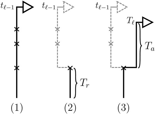
![Comparison of the accuracy of various conditional sampling distributions relative to $\batchmode \documentclass[fleqn,10pt,legalpaper]{article} \usepackage{amssymb} \usepackage{amsfonts} \usepackage{amsmath} \pagestyle{empty} \begin{document} \(\mathrm{{\hat{{\pi}}}}_{\mathrm{SMC-R}}\) \end{document}$ (see Figure 3 for the accuracy of $\batchmode \documentclass[fleqn,10pt,legalpaper]{article} \usepackage{amssymb} \usepackage{amsfonts} \usepackage{amsmath} \pagestyle{empty} \begin{document} \(\mathrm{{\hat{{\pi}}}}_{\mathrm{SMC-R}}\) \end{document}$). A and B illustrate that the improvement in accuracy of $\batchmode \documentclass[fleqn,10pt,legalpaper]{article} \usepackage{amssymb} \usepackage{amsfonts} \usepackage{amsmath} \pagestyle{empty} \begin{document} \(\mathrm{{\hat{{\pi}}}}_{\mathrm{SMC}\left(d\right)}\) \end{document}$ over $\batchmode \documentclass[fleqn,10pt,legalpaper]{article} \usepackage{amssymb} \usepackage{amsfonts} \usepackage{amsmath} \pagestyle{empty} \begin{document} \(\mathrm{{\hat{{\pi}}}}_{\mathrm{LS}}\) \end{document}$ and $\batchmode \documentclass[fleqn,10pt,legalpaper]{article} \usepackage{amssymb} \usepackage{amsfonts} \usepackage{amsmath} \pagestyle{empty} \begin{document} \(\mathrm{{\hat{{\pi}}}}_{\mathrm{FD}}\) \end{document}$ is amplified as the number of loci k increases and that both $\batchmode \documentclass[fleqn,10pt,legalpaper]{article} \usepackage{amssymb} \usepackage{amsfonts} \usepackage{amsmath} \pagestyle{empty} \begin{document} \(\mathrm{{\hat{{\pi}}}}_{\mathrm{LS}}\) \end{document}$ and $\batchmode \documentclass[fleqn,10pt,legalpaper]{article} \usepackage{amssymb} \usepackage{amsfonts} \usepackage{amsmath} \pagestyle{empty} \begin{document} \(\mathrm{{\hat{{\pi}}}}_{\mathrm{FD}}\) \end{document}$ produce significantly smaller values than $\batchmode \documentclass[fleqn,10pt,legalpaper]{article} \usepackage{amssymb} \usepackage{amsfonts} \usepackage{amsmath} \pagestyle{empty} \begin{document} \(\mathrm{{\hat{{\pi}}}}_{\mathrm{SMC-R}}\) \end{document}$ (and $\batchmode \documentclass[fleqn,10pt,legalpaper]{article} \usepackage{amssymb} \usepackage{amsfonts} \usepackage{amsmath} \pagestyle{empty} \begin{document} \(\mathrm{{\hat{{\pi}}}}_{\mathrm{SMC}}\) \end{document}$). For θ0 = 0.01 and ρ0 = 0.05, we used the methodology described in the text to sample 250 conditional configurations with n = 10 haplotypes and k loci. (A) Absolute log-ratio error. (B) Signed log-ratio error.](https://oup.silverchair-cdn.com/oup/backfile/Content_public/Journal/genetics/187/4/10.1534_genetics.110.125534/6/m_1115fig4a.jpeg?Expires=1716324514&Signature=mcMr3PMn2evFvw2iZ-GkiA-L4PGPTPgCwJJudTpd0-WoDG88CsilhxGI6AALO2GsX813Bwm8r2ip81n2Sd~KBEQs5asr1EDHEwu7QUIkD7gHkiZie9tkJwXXFAIVbXr2rVIATEPPD3cZoMcVfoUzguIfOTR-KeuUexIBWTRLCKO~27M84i0qL67OE007~TRPi6OpJN6u0Qnmvp~KnGCJ1g2WiVr9jULEr5xQlQ-BQZHKRGpcHpSmuBPPnHHy5FuDYK~Mudgmrg-BaQPuy~AW5Fl5VhUNbPQtBcW1-kpSm7IK58vS2SllwD-Pkn6dHZMJHz4vo9rn74Ut93RC-JadDw__&Key-Pair-Id=APKAIE5G5CRDK6RD3PGA)
![Comparison of the accuracy of various conditional sampling distributions relative to $\batchmode \documentclass[fleqn,10pt,legalpaper]{article} \usepackage{amssymb} \usepackage{amsfonts} \usepackage{amsmath} \pagestyle{empty} \begin{document} \(\mathrm{{\hat{{\pi}}}}_{\mathrm{SMC-R}}\) \end{document}$ (see Figure 3 for the accuracy of $\batchmode \documentclass[fleqn,10pt,legalpaper]{article} \usepackage{amssymb} \usepackage{amsfonts} \usepackage{amsmath} \pagestyle{empty} \begin{document} \(\mathrm{{\hat{{\pi}}}}_{\mathrm{SMC-R}}\) \end{document}$). A and B illustrate that the improvement in accuracy of $\batchmode \documentclass[fleqn,10pt,legalpaper]{article} \usepackage{amssymb} \usepackage{amsfonts} \usepackage{amsmath} \pagestyle{empty} \begin{document} \(\mathrm{{\hat{{\pi}}}}_{\mathrm{SMC}\left(d\right)}\) \end{document}$ over $\batchmode \documentclass[fleqn,10pt,legalpaper]{article} \usepackage{amssymb} \usepackage{amsfonts} \usepackage{amsmath} \pagestyle{empty} \begin{document} \(\mathrm{{\hat{{\pi}}}}_{\mathrm{LS}}\) \end{document}$ and $\batchmode \documentclass[fleqn,10pt,legalpaper]{article} \usepackage{amssymb} \usepackage{amsfonts} \usepackage{amsmath} \pagestyle{empty} \begin{document} \(\mathrm{{\hat{{\pi}}}}_{\mathrm{FD}}\) \end{document}$ is amplified as the number of loci k increases and that both $\batchmode \documentclass[fleqn,10pt,legalpaper]{article} \usepackage{amssymb} \usepackage{amsfonts} \usepackage{amsmath} \pagestyle{empty} \begin{document} \(\mathrm{{\hat{{\pi}}}}_{\mathrm{LS}}\) \end{document}$ and $\batchmode \documentclass[fleqn,10pt,legalpaper]{article} \usepackage{amssymb} \usepackage{amsfonts} \usepackage{amsmath} \pagestyle{empty} \begin{document} \(\mathrm{{\hat{{\pi}}}}_{\mathrm{FD}}\) \end{document}$ produce significantly smaller values than $\batchmode \documentclass[fleqn,10pt,legalpaper]{article} \usepackage{amssymb} \usepackage{amsfonts} \usepackage{amsmath} \pagestyle{empty} \begin{document} \(\mathrm{{\hat{{\pi}}}}_{\mathrm{SMC-R}}\) \end{document}$ (and $\batchmode \documentclass[fleqn,10pt,legalpaper]{article} \usepackage{amssymb} \usepackage{amsfonts} \usepackage{amsmath} \pagestyle{empty} \begin{document} \(\mathrm{{\hat{{\pi}}}}_{\mathrm{SMC}}\) \end{document}$). For θ0 = 0.01 and ρ0 = 0.05, we used the methodology described in the text to sample 250 conditional configurations with n = 10 haplotypes and k loci. (A) Absolute log-ratio error. (B) Signed log-ratio error.](https://oup.silverchair-cdn.com/oup/backfile/Content_public/Journal/genetics/187/4/10.1534_genetics.110.125534/6/m_1115fig4b.jpeg?Expires=1716324514&Signature=OfOJd5~LzOQRU7zTi5Bk~hUUVqMUSO9UrW-Pi12HvJgWddFUQyseVCMaMlELR2tvceSaCX5FpZ5EzSaQyGhid~iR5V3Huz8bI2TnDrv8K7GtnG25goBaHdqiXMZHm5hzmbczHh8mpvkS9Wq3cHye701nhm0rswO5LxxkqBcXhHWqIqex8oZpoinSaf9iIqcwoOm~VSMJ2HEcoIoWkLaFovukY8OXGB532Ip3xH1O0S4r~xgoAqxIBxKHryw-h1HQvq-~TTmTeiKwayuxmP7oSOPbv0NZmjWdJye0-WhCrf1878Od-PMB9UKlvbMa2RfaNETDJ1MMStGS4oJl8UobZA__&Key-Pair-Id=APKAIE5G5CRDK6RD3PGA)
![Illustration of the relationship between various CSDs. The CSD at the head of each arrow can be seen as an approximation to the CSD at the tail. Each arrow is also annotated with a (short) description of this approximation. The CSDs below the dashed line can be cast as an HMM: Those above the dotted line (including a continuous-state version of $\batchmode \documentclass[fleqn,10pt,legalpaper]{article} \usepackage{amssymb} \usepackage{amsfonts} \usepackage{amsmath} \pagestyle{empty} \begin{document} \(\mathrm{{\hat{{\pi}}}}_{\mathrm{FD}}\) \end{document}$, which we denote $\batchmode \documentclass[fleqn,10pt,legalpaper]{article} \usepackage{amssymb} \usepackage{amsfonts} \usepackage{amsmath} \pagestyle{empty} \begin{document} \(\mathrm{{\hat{{\pi}}}}_{\mathrm{FD-C}}\) \end{document}$) have a continuous and infinite state space, while those below have a finite and discrete state space and are therefore amenable to simple dynamic programming algorithms. For more thorough descriptions of each approximation, see the main text and also Paul and Song (2010). Recall in particular that the equality $\batchmode \documentclass[fleqn,10pt,legalpaper]{article} \usepackage{amssymb} \usepackage{amsfonts} \usepackage{amsmath} \pagestyle{empty} \begin{document} \(\mathrm{{\hat{{\pi}}}}_{\mathrm{SMC}}{=}\mathrm{{\hat{{\pi}}}}_{\mathrm{PS,1}}\) \end{document}$ holds only for conditionally sampling a single haplotype.](https://oup.silverchair-cdn.com/oup/backfile/Content_public/Journal/genetics/187/4/10.1534_genetics.110.125534/6/m_1115fig5.jpeg?Expires=1716324514&Signature=pxapcdNZ17EY~8~6duqfbTn7BE2ScwVpOw~TyYpaS-7Ta45FLbZ~ig3rAJdi5jQBpot6X6rlfYEWfrKXmVq~agUJGwlXeScu8PTioQDzsH6vNdoIEp6BYEqm3j6kZ3NafAiKfx~N0ovfYKh5vwvpO6bl4nAmyyI3FL7lQffEDb3WpI8KMPkdetsaKKLm9UMNAd9E6d585n3mx51NUG8VIQsqEizflSEJqCU5bRBY~lAJO2PbmuT~pQ9EUWZc0jZbY5mS61nqvoJPylNFRL3zIFi6BIjZQ8d7Op1TuVHcMQJa9hw4nQ~0gxNIh9YZIn~RvTMXD3Ai2DYMbXcrViN-Eg__&Key-Pair-Id=APKAIE5G5CRDK6RD3PGA)
