


Abstract
We propose a novel approximate-likelihood method to fit demographic models to human genomewide single-nucleotide polymorphism (SNP) data. We divide the genome into windows of constant genetic map width and then tabulate the number of distinct haplotypes and the frequency of the most common haplotype for each window. We summarize the data by the genomewide joint distribution of these two statistics—termed the HCN statistic. Coalescent simulations are used to generate the expected HCN statistic for different demographic parameters. The HCN statistic provides additional information for disentangling complex demography beyond statistics based on single-SNP frequencies. Application of our method to simulated data shows it can reliably infer parameters from growth and bottleneck models, even in the presence of recombination hotspots when properly modeled. We also examined how practical problems with genomewide data sets, such as errors in the genetic map, haplotype phase uncertainty, and SNP ascertainment bias, affect our method. Several modifications of our method served to make it robust to these problems. We have applied our method to data collected by Perlegen Sciences and find evidence for a severe population size reduction in northwestern Europe starting 32,500–47,500 years ago.
A major goal of evolutionary genetics is to infer the demographic history of a population. This is traditionally done by fitting a population genetic model to sequence data taken from a sample of individuals. The population genetic model often includes parameters allowing for changes in population size or population structure with or without migration. Such parameters are interesting in their own right, but are critical to define a proper “null model” that can be used to find “unusual” genes that may be targets of positive or negative selection (Jensen et al. 2005). Additionally, a proper demographic model is important for assessing genomewide patterns of positive and negative selection (Boyko et al. 2008; Lohmueller et al. 2008).
Methods have been developed that make full use of sequence data to infer demographic parameters (Griffiths and Tavaré 1994; Kuhner et al. 1995). These methods are computationally intensive and are impractical for all but the smallest data sets. Thus, researchers have turned to methods based on summary statistics (reviewed in Marjoram and Tavaré 2006). Summary statistics can be quickly calculated from the data and then be used to infer model parameters using either a likelihood or approximate Bayesian computation (ABC) framework (for example, Wall 2000a; Fagundes et al. 2007). The key for successful application of this approach is to find summaries of the data that contain enough information about the demographic parameters of interest. One of the most successfully used summary statistics for population genetic inference, the site frequency spectrum (SFS) (Nielsen 2000; Adams and Hudson 2004; Caicedo et al. 2007; Hernandez et al. 2007b), is a sufficient statistic for the full data if the single-nucleotide polymorphisms (SNPs) are unlinked. However, in reality, all SNPs are not unlinked. The amount of information in the data lost by ignoring the correlations among SNPs, or linkage disequilibrium (LD), in demographic inference is an open question, but recent theoretical work suggests that it may be nonnegligible (Myers et al. 2008).
An additional complication to using the SFS for demographic inference is that many genomewide genetic variation data sets in humans contain SNPs that were discovered through sequencing a small number of individuals. The discovered SNPs were then genotyped in a larger set of individuals, sometimes in a different population than was used for SNP discovery. Since this SNP discovery process will lead to preferential sampling of intermediate-frequency alleles, the SFS computed from SNP genotype data will differ substantially from the true SFS (Nielsen et al. 2004; Clark et al. 2005). Progress has been made to analytically correct the SFS for ascertainment bias when the SNP discovery process is known (Nielsen et al. 2004), but often this is not the case. More problematic is the situation where SNPs were discovered by resequencing individuals in one population, but then are genotyped in a second population. It remains an open question as to how well the SNPs discovered in the first population are representative of genetic diversity in the second population. Several authors have suggested that statistics based on combinations of multiple SNPs, or haplotypes, will be less susceptible to ascertainment bias than single-SNP frequencies or heterozygosities (Conrad et al. 2006). However, while this suggestion is encouraging, as yet there has not been extensive investigation into the precise ascertainment conditions under which this is true.
It is known that haplotype patterns and LD can be affected by both recombination and demographic history (Pritchard and Przeworski 2001), making these measures useful statistics for inference. Many recent studies have assumed a demographic model (often the standard neutral model) and then used either LD or haplotype patterns to estimate recombination rates (Wall 2000a; Hudson 2001; Li and Stephens 2003; McVean et al. 2004; Myers et al. 2005). Other studies have taken the opposite approach and assumed that the recombination rate is known and then used LD or haplotype patterns to estimate demographic parameters (Reich et al. 2001; Innan et al. 2005; Voight et al. 2005; Schaffner et al. 2005; Leblois and Slatkin 2007; Tenesa et al. 2007). The way in which haplotype information has been used for demographic inference is quite variable among studies. For example, Reich et al. (2001) examined how well several different demographic models predicted the observed decay of pairwise LD in humans, rather than estimating the model parameters. Francois et al. (2008) and Thornton and Andolfatto (2006) used ABC to estimate model parameters in Arabidopsis and Drosophila, respectively. However, summaries based on the distribution of the number of haplotypes were only one of several summary statistics considered, and it is unclear how much information came from the haplotype information vs. the other single-SNP diversity measures. While Anderson and Slatkin (2007) and Leblois and Slatkin (2007) developed methods that use haplotype information exclusively to fit a population split followed by growth model, their model is quite restrictive and allows inference only of one free parameter, the number of founding lineages. Thus, there has not been a systematic investigation as to the utility of haplotype information for inference in general, parameter-rich models, such as those involving population expansions and bottlenecks.
In this article we propose an approximate-likelihood method to estimate parameters in complex demographic models from genomewide SNP genotype (rather than full resequencing) data, using the joint distribution of the number of haplotypes and frequency of the most common haplotype in windows across the genome. We provide extensive simulations evaluating the performance of our method for growth and bottleneck models. These results indicate that a great deal of information regarding demographic history is captured by these two summary statistics. We also extensively test the robustness of our method to many practical problems with genetic data sets in humans. Specifically, we show that for many realistic SNP discovery protocols and levels of population divergence, our method is relatively robust to SNP ascertainment bias. We also found that our method is sensitive to recombination rate variation across the genome (as many haplotype-based summaries will be), and we incorporate a model of recombination rate variation into the inference scheme. Finally, since haplotype phase is often ambiguous, we provide a practical approach to circumvent this problem. We applied our method to genomewide SNP genotype data generated by Perlegen Sciences (Hinds et al. 2005). Using the CEU sample (consisting of individuals from Utah with northwestern European ancestry), we find evidence for a recent population bottleneck in northwestern Europe.
METHODS
Summary statistics:
We summarize the genomewide data by the joint distribution of two haplotype statistics calculated from windows across the genome. Our method requires that we have a genetic map of the organism in question. Using this map, we divide the genome into windows of fixed genetic map distance, cwindow. The parameter cwindow is tunable to the diversity and recombination rates of the organism under study. We chose to divide the genome into nwindow nonoverlapping windows using genetic map distance so that each window will have the same expected amount of recombination within it and, consequently, the same expected number of haplotypes (Wall 2000a).
In many genomewide SNP data sets, some parts of the genome will have a small number of SNPs while other areas will contain many SNPs. In principle, while this could be due to mutation rate variation across the genome, variations in the time to the most recent common ancestor, or random chance, another likely explanation is ascertainment bias—some parts of the genome were more extensively screened for SNPs than others and consequently have more SNPs. Thus, we do not want our method to use any information about the number of SNPs within a given window. To ensure that all windows of the genome have the same number of SNPs, we select a subset of nsnp SNPs for each window of the genome. Again, nsnp is a function of the size of the windows as well as the SNP density. Another complicating factor is that SNPs may not have been discovered from the population under study, but instead from a second population. Since rare SNPs are more likely to be population specific, and consequently not equally ascertained in all populations, we include only those SNPs with minor allele frequency (MAF) ≥10%.
Having selected a subset of intermediate-frequency SNPs from each window, we can compute the number of distinct haplotypes as well as the count of the most common haplotype in a sample of n chromosomes. The HCN statistic is the genomewide joint distribution of these two statistics. Specifically, let
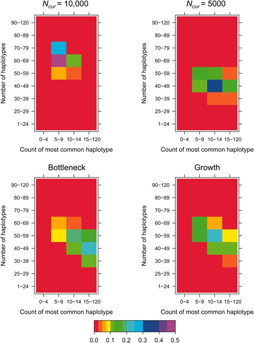
Examples of the HCN statistic for different demographic models. The color of each cell in a matrix denotes the proportion of simulated windows having the particular number of haplotypes and frequency of the most common haplotype. Approximately 3000 windows were simulated for each demographic model with nsnp = 25, cwindow = 0.25 cM. The parameters for the bottleneck model are Ncur = Nanc = 10,000, Nmid = 1000, and tcur = tmid = 800 generations. The parameters for the growth model are Ncur = 10,000, Nmid = 1000, and tcur = 800 generations.
We chose to use the number of haplotypes as a summary statistic because it is a sufficient statistic for the population mutation rate
The HCN statistic contains no information about how different haplotypes within a window are from each other. To add this information, we also considered another summary statistic Hpair, the distribution across the genome of the average number of pairwise differences between haplotypes. For all
Demographic models:
We consider two different single-population demographic models. These models and their associated parameters are shown in Figure 2. Figure 2A shows a two-epoch model that is used for modeling population growth. Here there are three parameters to estimate: the current population size, Ncur; the ancestral population size, Nmid; and the time that growth has occurred, tcur. Figure 2B shows a three-epoch model that has five free parameters: the current population size, Ncur; the population size during the bottleneck, Nmid; the ancestral population size, Nanc; the time when the bottleneck started (going backward in time), tcur; and the duration of the bottleneck, tmid. All times are in units of generations. We note that although these models (and all models in population genetics) are arbitrary simplifications of the true demographic history, the hope is that they capture some essential features of population history.
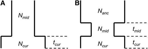
Demographic models considered. Relevant free parameters are shown in each diagram. (A) Two-epoch model; (B) three-epoch model.
Fitting models to data:
Since we select nsnp SNPs from each window,
We optimize the approximate-likelihood function described above using a grid search since we are approximating the likelihoods by simulation and the simulation variance may be nonnegligible, misleading deterministic hill-climbing approaches. The number of grid points and number of simulation replicates used to maximize the approximate-likelihood function vary among analyses and are given below.
Since variation in recombination rates at a fine scale can affect the HCN statistic, we have added a model of recombination hotspots into our inference method. We describe the parameters used for specific instances below. Since each window of the genome corresponds to the same genetic map distance (cwindow), the number of base pairs per window will differ among windows. In our simulations to find
Simulations to evaluate performance:
We tested the performance of our method by simulating data under three different demographic models: (1) ancient population growth, (2) recent population growth, and (3) a recent population bottleneck. The parameter values for these models are shown in Figures 3–Figures 6. These models were chosen because of their relevance to human demographic history. For each model we simulated data sets (500 for models assuming uniform recombination rates and 100 for models with recombination hotspots), each consisting of 2000 independent 250-kb windows in a sample of 40 chromosomes where μ = 1 × 10⁻⁸/bp/generation. Note that when generating test data sets, we placed a Poisson number of mutations onto the genealogies in the usual fashion (Hudson 1983), rather than using the fixed S approach as we did for the simulations used to estimate
For all data sets and demographic models, the total amount of recombination within each window simulated was 0.25 cM (i.e., cwindow = 0.25 cM). However, we also considered a model with five recombination hotspots present at random locations throughout each window. Each hotspot was 2 kb in size. The recombination rate (centimorgans per base pair) of each hotspot was drawn from a gamma distribution (shape = 0.5, scale = 2 × 10⁻⁶). We then rescaled the recombination rate of each hotspot such that 80% of the total amount of recombination in the window occurs within hotspots. We then assumed this model of recombination hotspots when inferring demographic parameters. The test data sets were generated using the program msHOT (Hellenthal and Stephens 2007).
Our method assumes that all windows in the genome are independent of each other. To assess the performance of our method when the windows are not independent, we simulated an additional 500 data sets using the same bottleneck model with
While for most of the simulations we assumed that there was no error in estimated recombination rates (i.e.,
Due to differences between the true HCN statistic and the HCN statistic constructed from phase-inferred haplotypes (Figure S2 and File S1), it is important to incorporate the phasing process into the inference. To do this, we suggest using the same phasing method that was used on the actual data to “phase” the simulated data used to estimate
Since we found that the HCN statistic constructed using SNPs that were discovered in a SNP discovery sample ≥8 chromosomes was very similar to the HCN statistic with complete SNP ascertainment (Figure S3, Figure S4, Figure S5, Table S1, and File S1), we examined how ascertainment bias affected parameter estimates. Specifically, for the bottleneck model described above, we simulated a genotype sample of n = 40 and an additional SNP discovery sample of 6 chromosomes. Since the Perlegen SNPs were discovered using a multiethnic panel (Hinds et al. 2005), we included a SNP discovery sample of an additional 6 chromosomes from a second population (Ncur = 10,000) that 5000 generations ago split from the population that underwent the bottleneck. To construct the HCN statistic from these simulated data sets, we considered only SNPs with MAF
Analysis of Perlegen data:
We applied our method to fit a bottleneck model to the CEU population genotyped by Perlegen Sciences (Hinds et al. 2005). We chose to use this population since there is previous evidence of a bottleneck in this population (e.g., Marth et al. 2004; Voight et al. 2005), and all SNPs that were discovered by the Perlegen resequencing arrays were later genotyped in the CEU sample, without regard to LD status. We note that HapMap phase II specifically did not genotype SNPs that were in high LD in the Perlegen study, and this ascertainment criterion complicates the analysis of those data (see discussion). We considered only autosomal (not X chromosome or mtDNA) SNPs with MAF
We then set cwindow = 0.25 cM and nsnp = 20. We used the LDhat genetic map (International Hapmap Consortium 2007) to define windows since the deCODE map (based on pedigrees; Kong et al. 2002) does not have sufficient resolution for the scale of 0.25 cM (Myers et al. 2005). Since the quality of the genetic map used to divide the genome into windows can affect the inference, we drew
We used a hotspot model similar to that of Schaffner et al. (2005; termed the “Schaffner hotspot model”). All hotspots had width of 2 kb. For each simulated window, hotspots occurred at random intervals drawn from a gamma distribution (shape = 0.3, scale = 8500/0.3), giving a mean spacing of 8.5 kb (variance of ∼2.41 × 10⁸). Then the recombination rate (cM/2 kb) of each hotspot was drawn from another gamma distribution (shape = 0.3, scale
In addition to the Schaffner hotspot model described above, we also directly used the estimated fine-scale LDhat genetic map (International Hapmap Consortium 2007) as a guide to how recombination rates vary within windows (termed the “empirical hotspot” model). To do this, for each simulation replicate to estimate
The grid to optimize the five-dimensional approximate-likelihood function consisted of 85,536 points for the Schaffner hotspot model and 101,088 points for the empirical hotspot model. We used 12,500 simulation replicates for all points, 105 replicates for at least the top 4000 points, and finally 106 replicates for at least the top 500 points. We found approximate 95% confidence intervals (C.I.'s) for single parameters using asymptotic theory (i.e., the C.I. included points <1.92 log-likelihood units from the maximum), with linear interpolation of the profile-likelihood curve to find points not directly simulated.
RESULTS
Performance on simulated data:
Figure 3 shows the distribution of the approximate MLEs of the three growth model parameters for simulated data sets under ancient growth (solid bars) and recent growth (open bars). In both cases, the method is relatively unbiased for all three parameters. For ancient growth, Ncur is estimated most accurately and tcur the least. For recent growth, all three parameters are equally accurate, although for any given parameter, the MLE is the true value ∼40% of the time. Note that the variance in the distribution of MLEs for tcur is much higher for ancient growth as compared to recent growth (making it the least precise as well as the least accurate). Table 1 shows that for both growth scenarios in 100% of the data sets, the true parameter values were within the asymptotic 95% C.I.'s (<3.9 log-likelihood units) around the MLEs. Additionally, in >95% of the data sets, the one-dimensional 95% C.I.'s for all three parameters from the profile-likelihood curves contain the true parameter values.
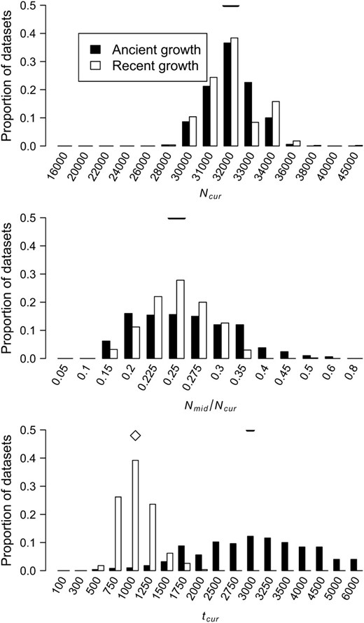
Distributions of MLEs of the three growth model parameters for simulated data sets under ancient growth and recent growth with uniform recombination (see methods). The true value of each parameter is denoted by the horizontal line in each section. Since tcur differs between the two growth models, the true value of tcur is denoted by an open diamond for recent growth and a horizontal line for ancient growth.
Comparison of MLEs to the true parameter values for simulated data sets
Model | Mean llMLEs − llTrutha | Max llMLEs − llTruthb | % MLEs = truthc | Coverage of multidimensional 95% C.I.'sd | Coverage of one- dimensional 95% C.I.'se | % points outside 95% C.I.'sf |
|---|---|---|---|---|---|---|
| Ancient growth | ||||||
\({\hat{c}}_{\mathrm{window}}{=}c_{\mathrm{window}}{=}0.25\) cM | 0.631 | 3.47 | 3.0 | 100.0 | 99.87 | 94.79 |
| Recent growth | ||||||
\({\hat{c}}_{\mathrm{window}}{=}c_{\mathrm{window}}{=}0.25\) cM | 0.437 | 3.09 | 22.6 | 100.0 | 99.93 | 98.84 |
| Bottleneck | ||||||
\({\hat{c}}_{\mathrm{window}}{=}c_{\mathrm{window}}{=}0.25\) cM | 0.363 | 6.31 | 47.4 | 99.8 | 99.52 | 99.87 |
| Hotspotsg | 0.505 | 3.43 | 17.0 | 100.0 | 99.80 | 99.65 |
| Linkage | 0.732 | 8.30 | 29.8 | 99.4 | 98.48 | 99.87 |
\({\hat{c}}_{\mathrm{window}}{=}0.25\) cM, \(c_{\mathrm{window}}{\sim}\mathrm{gamma}\) | 136.685 | 179.07 | 0.0 | 0.0 | 8.36 | 99.98 |
\({\hat{c}}_{\mathrm{window}}\mathrm{{\sim}}c_{\mathrm{window}}{\sim}\mathrm{gamma}\) | 0.623 | 6.54 | 26.4 | 99.6 | 99.40 | 99.72 |
| Clark's phasing algorithmh | 0.779 | 4.90 | 19.8 | 100.0 | 99.96 | 99.43 |
| Ascertainment bias | 1.998 | 12.65 | 14.6 | 94.0 | 97.64 | 99.86 |
The average overall data sets of the log-likelihood at the MLEs minus the log-likelihood of the true demographic parameters.
The maximum distance between the log-likelihood at the MLEs and the log-likelihood of the true demographic parameters.
The proportion of data sets where the MLEs for all parameters were the true demographic parameters.
The proportion of data sets where the true parameter values were <3.9 or <5.5 log-likelihood units from the MLEs, for the growth and bottleneck models, respectively.
The proportion of data sets where the true value of each parameter was <1.92 log-likelihood units from the MLE using the profile log-likelihood curve, averaged over three or five parameters for the growth and bottleneck models, respectively.
The fraction of grid points (see results) having a log-likelihood >3.9 or >5.5 log-likelihood units, for the growth and bottleneck models, respectively, from the MLEs.
Each window has five recombination hotspots, but for the whole window
Haplotype phase was inferred in the test data sets and simulations to estimate
We also estimated the five parameters for a bottleneck model in simulated data sets. Figure 4 shows the distribution of the MLEs for the five bottleneck parameters. For the case of uniform recombination and
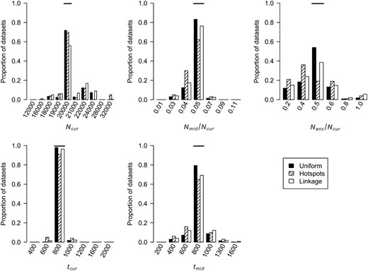
Distributions of MLEs of the five bottleneck model parameters for simulated data sets under uniform recombination, under hotspots, and where some windows in the simulated data sets are linked to one another (see methods). The true value of each parameter is denoted by the horizontal line in each section.
We next evaluated whether our method could accurately estimate demographic parameters in the presence of recombination hotspots (see methods for the recombination hotspot model used). Figure 4 shows that when properly modeling recombination hotspots, we are able to accurately estimate the five bottleneck model parameters. Note that the distributions of the MLEs for all parameters have larger variances than for the uniform recombination case. This pattern is due to the extra noise added by recombination hotspots. If a window of the genome has a low number of haplotypes and/or a high count of the most common haplotype, this could be due to demography (which is the only factor considered in the uniform recombination model) or due to SNPs falling in recombination coldspots. Consistent with this observation, Table 1 shows that a smaller proportion of the parameter space (99.65% vs. 99.87%) is >5.5 log-likelihood units from the MLEs when there are recombination hotspots, as compared to uniform recombination. Notably, however, the method still appears to be unbiased, and for all 100 data sets, the true parameter values are <5.5 log-likelihood units from the MLEs.
The simulations described above assumed that the windows in each data set were independent. In practice, the windows may be contiguous along the genome and thus are not independent. We examined the performance of our method on simulated data sets where some of the windows were linked. Figure 4 shows that the distributions of the MLEs for certain parameters have greater variance than when the windows are unlinked, which is not surprising since linked windows contain less information than independent windows. As shown in Table 1, in all cases except when errors in the genetic map are ignored or there is SNP ascertainment bias (see below), the true parameter values for >99% of the test data sets are within the asymptotic 95% C.I.'s (<3.9 and <5.5 log-likelihood units from the MLEs for growth and bottleneck models, respectively). This result suggests that the asymptotic C.I.'s may actually be conservative, since the true parameter values are contained within the interval >95% of the time. When examining data sets where some of the regions are linked, we find that for 99.4% of the time, the true values are <5.5 log-likelihood units from the MLEs (Table 1). Since in many cases, the 95% C.I.'s for individual parameters based on the profile log-likelihood curve also appeared conservative (Table 1), we assessed their coverage in the data sets with linkage. For each of the five parameters, the true parameter value is <1.92 log-likelihood units from the MLE in at least 96.8% of the data sets. These results suggest that for the level of nonindependence among windows, size of data sets, and parameter grid considered here, the asymptotic 95% C.I.'s remain conservative.
The above simulations assumed that
![Distributions of MLEs of the five bottleneck model parameters for simulated data sets where there are errors in the genetic map. $\batchmode \documentclass[fleqn,10pt,legalpaper]{article} \usepackage{amssymb} \usepackage{amsfonts} \usepackage{amsmath} \pagestyle{empty} \begin{document} \({\hat{c}}_{\mathrm{window}}{=}0.25{\,}\mathrm{cM,}c_{\mathrm{window}}{\sim}\mathrm{gamma}\) \end{document}$ denotes the case where there are errors in the estimated genetic map that are ignored when performing the inference. $\batchmode \documentclass[fleqn,10pt,legalpaper]{article} \usepackage{amssymb} \usepackage{amsfonts} \usepackage{amsmath} \pagestyle{empty} \begin{document} \({\hat{c}}_{\mathrm{window}}\mathrm{{\sim}}c_{\mathrm{window}}\mathrm{{\sim}gamma}\) \end{document}$ denotes the case where we allow for errors in the genetic map when conducting the inference. The true value of each parameter is denoted by the horizontal line in each section.](https://oup.silverchair-cdn.com/oup/backfile/Content_public/Journal/genetics/182/1/10.1534_genetics.108.099275/7/m_217fig5.jpeg?Expires=1716437837&Signature=NzP3UUIa-azgow7ZApiScmMrRYKA1qcWtDTUcemoUl8KNXyGeUGHfMK7peanXs0nWIBhFYDFpMVPU4SbGoGZ19z8FLZ8fHVfMjagqupwnk-bnVhCG6U-4eWzy9FWaBfPATa6eZJyuc3YuHImqOYuKoaOWRhqQ9sZJV1OhTjs-J34G75O6Y3tuC3NFeRJ2t7~uEdc6r0PMICFr-ug4snOYsmX5w~B9iyp14FD7neT8x8FpuzmxWLG9tkvIouxPtWlVyuN2O6-yEI5UdqcWz6Y8WhfUFEUWgRc5XcGIJ684EBJePAA2cGN7Ei3GZaPXS39kWY1ITb2eY2ZbRDsZhxH7Q__&Key-Pair-Id=APKAIE5G5CRDK6RD3PGA)
Distributions of MLEs of the five bottleneck model parameters for simulated data sets where there are errors in the genetic map.
To properly correct for errors introduced from inferring haplotype phase, we decided to phase the simulations used to estimate
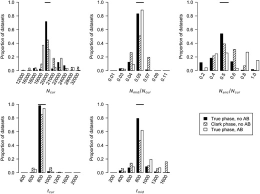
Distributions of MLEs of the five bottleneck model parameters for simulated data sets when phasing genotype data using Clark's phasing algorithm or there is SNP ascertainment bias (AB) (see methods). The true value of each parameter is denoted by the horizontal line in each section.
To determine if we could accurately estimate bottleneck parameters in the presence of SNP ascertainment bias, we simulated data sets where the nsnp = 20 SNPs for each window were picked from those SNPs with MAF
Inference of bottleneck parameters for the Perlegen CEU population:
We fit the five-parameter bottleneck model to the Perlegen CEU population. Table 2 shows the MLEs and ∼95% C.I.'s for the five parameters when using both the Schaffner model of recombination hotspots and the empirical hotspot model based on the LDhat genetic map. Figure S8 shows that for both hotspot models, the HCNs generated using the MLE parameter estimates match the observed CEU HCN quite well. The current population size is estimated to be ∼10,000 when using both recombination models. There was a severe population size reduction (∼4.2–6.6% of the current size) lasting 260–552 generations (see Figure S9 for the two-dimensional profile-likelihood surface). The bottleneck ended (forward in time) ∼1017–1437 generations ago.
Inferred bottleneck parameters for the CEU data set
Schaffner hotspot modela | Empirical hotspot modelb | |||
|---|---|---|---|---|
| Parameter | MLE | 95% C.I. | MLE | 95% C.I. |
| Ncur | 10,000 | 9,315–10,665 | 10,000 | 9,440–11,454 |
| Nmid/Ncur | 0.055 | 0.052–0.064 | 0.05 | 0.042–0.066 |
| Nanc/Ncur | 0.8 | 0.70–?c | 0.8 | 0.66–0.97 |
| tcur | 1,100 | 1,017–1,140 | 1,200 | 1,086–1,437 |
| tmid | 400 | 360–475 | 300 | 260–552 |
MLEs and ∼95% C.I.'s from the profile-likelihood curves for the five-parameter bottleneck model are shown.
The hotspot model is similar to that described by Schaffner et al. (2005) (see methods).
The hotspot model is based directly on the LDhat genetic map.
We did not estimate an upper boundary on the C.I. since the profile-likelihood surface for Nanc/Ncur is relatively flat from 0.8 to 1.0 and we did not consider points >1.0 (Figure S11).
On the basis of the two-dimensional profile-likelihood surface (Figure S10), we estimate that the bottleneck began (tcur + tmid) 1500 generations ago—37,500 years, assuming 25 years/generation when using either hotspot model. Notably, the oldest start time within the asymptotic 95% C.I. (3 log-likelihood units, for 2 d.f.) is 1600 generations, or 40,000 years for the Schaffner hotspot model, and 1900 generations (47,500 years) for the empirical hotspot model.
One potential concern with using SNPs from the Perlegen SNP discovery project is that it contains a lot of missing data, resulting in some fraction of SNPs having been discovered in a smaller sample. To determine what effect this had on the inference of the bottleneck parameters, we examined the depth of the SNP discovery panel for the 615,415 SNPs used in constructing the HCN statistic used for demographic inference in the Perlegen CEU sample. We found that 11.8% of these SNPs were discovered by comparing fewer than eight chromosomes. We removed these SNPs and recomputed the HCN statistic from the Perlegen CEU data (now with 8174 windows) and reestimated the bottleneck parameters using the Schaffner recombination hotspot model. We found identical MLEs for the parameters as in our original analysis.
DISCUSSION
We have proposed a flexible approximate-likelihood method to estimate demographic parameters using haplotype summary statistics. We have shown that accurate estimates of demographic parameters can be made using genomewide SNP data sets of practical size. To the best of our knowledge, this is one of the first studies to estimate parameters in a demographic model in a likelihood framework using haplotype patterns from genomewide SNP genotype data. Furthermore, we have addressed many complications that arise in the analysis of genomewide data, such as recombination rate heterogeneity, errors in the estimated genetic map, haplotype phase uncertainty, and ascertainment bias. Provided that good genetic maps are available, our method could be applied to SNP data from other species, such as dogs and cattle, to estimate domestication bottleneck parameters.
One of the major disadvantages of our approach is its dependence on accurately modeling the distribution of recombination rates across the genome. Our simulations have shown that errors in the genetic map can cause poor performance. Therefore, we suggest applying our method only when there is an accurate genetic map for the species in question. We suggest incorporating a distribution on
We also assume that the genetic map remains constant over time and is the same across populations. Recombination hotspots do not appear in the same locations in chimps and humans despite a high level of sequence identity (Ptak et al. 2005; Winckler et al. 2005). It has therefore been speculated that recombination hotspots are not permanent features of the genome and evolve on a timescale of at least tens of thousands of years (Jeffreys et al. 2005). However, it appears that the timescale over which many hotspots evolve is older than 100,000 years, and because this is long enough to alter patterns of LD, temporal changes in hotspots on this timescale will not have such a severe impact on our method. Hotspots that evolve over shorter timescales, or are population specific, may have a larger effect on our method. This effect is hard to quantify since the prevalence of rapidly evolving or population-specific hotspots, other than the existence of a few examples (Jeffreys et al. 2005; Clark et al. 2007), remains largely unknown. Encouragingly, a recent article (Hellenthal et al. 2006) found that genotype-specific recombination events would not substantially affect LD patterns, boding well for our method.
We have found that the HCN statistic constructed from computationally phase-inferred data differs from the true HCN. Simply treating the phase-inferred haplotypes as the true haplotypes will likely give biased parameter estimates. Thus, when analyzing data from unrelated individuals, it is important to consider errors induced in the phasing process. We suggest doing this by inferring phase for the coalescent simulations used to estimate HCN. Our simulations suggest that using Clark's phasing algorithm works well for this purpose. However, some information is lost by this procedure (Figure 6; Table 1), and we therefore recommend, where available, using data from trios, where haplotype phase can be inferred with great accuracy, to maximize the information in the data.
It has been suggested (Conrad et al. 2006) that haplotype statistics may be less susceptible to SNP ascertainment bias than statistics based upon SNP frequencies. Here we have extensively investigated whether this holds true for the HCN and Hpair statistics under a variety of demographic and ascertainment conditions. Encouragingly, we found that the HCN statistic is reasonably robust to SNP ascertainment bias provided that the SNP discovery sample is sufficiently deep. The reason for this is that we focus on subsets of common SNPs, rather than on rare SNPs. However, the Hpair statistic was very susceptible to ascertainment bias (Figure S1 and File S1), suggesting that all haplotype statistics are not equally affected by ascertainment bias, and it will be necessary to explicitly evaluate, as we have done here, whether ascertainment bias affects a particular haplotype statistic.
The sizes of the SNP discovery and genotype samples play an important role in determining the effect of ascertainment bias on the HCN statistic. Interestingly, generating the HCN from SNPs ascertained uniformly using two chromosomes of known ethnicity (as done by Keinan et al. 2007) would result in a very different HCN statistic from that expected without ascertainment bias (Figure S3, Figure S4, and Figure S5), which would result in biased inference. Although not considered here, it is in principle possible to estimate the expected HCN statistic conditional on this particular ascertainment strategy, and application of such an estimate would reduce this bias.
We have found that SNP discovery sample sizes of at least 12 total chromosomes should be sufficient to result in the HCN statistic from ascertained SNPs to match the expected HCN when considering genotype samples of 40 or 120 chromosomes. Furthermore, we have shown that our method can reliably infer several bottleneck parameters when SNPs were ascertained in this manner. As the SNP discovery sample size increases, performance of our method will continue to improve and become closer to that for the case of no ascertainment bias, since a larger SNP discovery sample will capture more of the SNPs in the genotype sample. These results are especially encouraging since Perlegen's SNP discovery effort used 20–50 chromosomes, where ∼12 chromosomes were of African-American ancestry, ∼12 chromosomes were of European ancestry, and the remainder were of Mexican-American, Asian-American, and Native American ancestry (Collins et al. 1998; Hinds et al. 2005).
Furthermore, we have found that the size of the SNP discovery sample is more important than whether or not the SNP ascertainment had been done in a particular population (see Figure S5). This suggests that SNPs ascertained in the Perlegen resequencing survey could be used to estimate demographic parameters in other populations not represented in the SNP discovery panel. It is worth noting that the two populations in our simulation study shown in Figure S5 split 5000 generations ago (125,000 years, assuming 25 years/generation) with no subsequent migration and are thus more differentiated than many actual non-African populations that could be studied empirically.
It is important to note that the type of ascertainment bias studied here is due to the preferential genotyping of common SNPs. In all the analyses presented here, we assume that the genotyped SNPs were selected without regard to physical or genetic distance or LD patterns. Such an assumption is reasonable for the analyses of the Perlegen data presented here since Perlegen attempted to genotype all of the SNPs found in their SNP discovery process (Hinds et al. 2005). The assumption is not valid, however, for many of the “SNP chips” that preferentially selected SNPs on the basis of physical distance (in the case of Affymetrix 500K) or LD patterns (in the case of the Illumina platform; Eberle et al. 2007). Since the SNPs on these platforms are not a random subset of the total variation, using our method on such data will likely give misleading results. In principle, it should be possible to modify our method to model the SNP selection process in the inference, which would allow our method to be applied to the large-scale SNP genotype data sets that have been collected, such as the HGDP data set (Jakobsson et al. 2008; Li et al. 2008).
For the analysis of the CEU data, we used two different models of recombination rate variation. Overall, the results using both models are qualitatively similar, suggesting that our method is somewhat robust to minor misspecification of the recombination hotspot model. We also find that the one-dimensional 95% C.I.'s from the profile-likelihood curves overlap for all five parameters estimated (Table 2; Figure S11). Nevertheless, the five-dimensional 95% C.I.'s do differ between the two recombination models, mainly due to the fact that tcur is greater under the empirical hotspot model than under the Schaffner hotspot model.
The time we inferred that the CEU bottleneck began (∼37,500 years ago) is too recent to coincide with the accepted dates for the out-of-Africa bottleneck, which is believed to have occurred 40,000–80,000 years ago (Reed and Tishkoff 2006). Thus, our estimate may coincide with an additional bottleneck associated with the founding of Europe, which likely took place 30,000–40,000 years ago (Barbujani and Goldstein 2004). Alternatively, our estimated start time of the bottleneck may represent an average time over several bottlenecks, including the out-of-Africa bottleneck and a more recent bottleneck, perhaps associated with the Last Glacial Maximum that began ∼18,000 years ago (Barbujani and Goldstein 2004). Further work considering multiple European populations and multiple bottlenecks may help resolve this question.
How do our estimates of the bottleneck parameters for the CEU match with published estimates? Voight et al. (2005) may not be directly comparable to our study since their analysis considered a southern European sample and ours used individuals with northwestern European ancestry, and differences in haplotype diversity between these two regions have been noted (Lao et al. 2008; Auton et al. 2009). Nevertheless, our estimates of tmid and Nmid/Ncur fall within their confidence regions. Their bottleneck start times (40,000 years) and current and ancestral population size estimates (∼10,000) also agree with ours. Our estimate of the time the bottleneck began is also consistent with that found using the decay of pairwise LD. Reich et al. (2001) found evidence for a bottleneck 800–1600 generations ago (our MLE is 1500 generations). We find evidence for a more severe bottleneck than previously estimated (Adams and Hudson 2004; Marth et al. 2004; Keinan et al. 2007), which could reflect the importance of considering LD-based information in the inference since these studies are all based on the frequency spectrum, and the other study that considers a summary of LD (Voight et al. 2005) cannot reject such a severe bottleneck. Alternatively, there could be some other important factors in European population history not captured by these simple bottleneck models that may affect the frequency spectrum and LD patterns differently. Finally, we cannot exclude the possibility that we have overestimated the bottleneck intensity due to greater heterogeneity in the recombination rate than what was included in our hotspot models. In short, improved confidence in the fine-scale genetic map will allow definitive ability to discriminate between these alternative scenarios.
While we have shown that haplotype statistics can be used to estimate demographic parameters from SNP genotype data, and it has been shown that the site frequency spectrum (SFS) will give misleading results when applied to genotype data without a correction for ascertainment bias (Nielsen et al. 2004; Clark et al. 2005), one important question is whether haplotype summary statistics will provide additional information that is important for inference when full genomewide resequencing data are available and it is possible estimate the SFS accurately. We examined whether the number of haplotypes and the count of the most common haplotype can discriminate between two different demographic models that have similar SFSs. We focused on a demographic model that included ancestral population structure since previous studies found that ancestral structure can result in an excess of long-range LD (Wall 2000b; Plagnol and Wall 2006). Specifically, we found that for certain subsets of the parameter space (the ms command lines giving the parameters used to generate Figure 7 are given as File S1), population growth with ancestral structure can create a similar SFS to that expected under population growth without ancestral structure. Close inspection of Figure 7 reveals a very slight uptick in the proportion of high-frequency derived SNPs in the population growth with structure SFS as compared to the growth without structure SFS, which is the expected signal of ancestral population structure. However, this effect is very subtle and in practice may be attributed to misidentification of the derived allele, rather than ancestral population structure (Hernandez et al. 2007a). Note that while the magnitudes of growth in the structure and panmictic cases are different, the growth with structure case still has an excess of low-frequency SNPs (Figure 7), which would often be interpreted as evidence for population growth. The inset in Figure 7 shows the count of the most common haplotype vs. the number of haplotypes for 10,000 windows simulated under the two demographic models described above. Note the growth with structure model has an excess of windows where the most common haplotype is at higher frequency and an excess of windows with a fewer number of haplotypes compared to the pure growth model. Thus, this is a case where two demographic models that cannot be readily differentiated on the basis of the SFS can be distinguished easily using haplotype patterns. The reason for this is as follows: population growth results in an excess of low-frequency SNPs, and for the parameters used here, population structure results in an excess of both low-frequency and high-frequency derived alleles. The resulting SFSs in Figure 7 have been affected by both these forces, but the excess of low-frequency SNPs is the predominant feature. Since ancestral population structure results in some genealogies having longer internal branches, any mutations occurring on these branches will be in LD with each other, leading to fewer distinct haplotypes in the sample and the most common haplotype occurring at higher frequency. Additionally, since the SFS treats all SNPs as being independent, haplotype patterns capture more information regarding the local genealogy within a window than the SFS does. In other words, many of the high-frequency derived SNPs in the sample are clustered in certain windows, but this pattern is missed in the SFS since it treats all SNPs as being exchangeable. Notably, summaries of the SFS performed on a local scale may be better at distinguishing these two models (Figure S12).
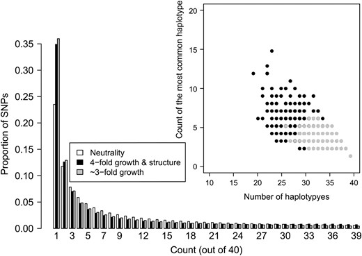
Comparison of the expected SFS for population growth with ancestral structure to that expected with just population growth. The inset shows the frequency of the most common haplotype vs. the number of haplotypes for each simulated window for the same two demographic models. Note that the SFSs for the two models appear similar, but that there is an excess of windows with fewer haplotypes and where the most common haplotype is at high frequency in the growth with ancestral structure model (see discussion).
It is important to point out that the HCN statistic has been designed to be used on ascertained SNP data, where the number of SNPs in a particular window of the genome is affected by the ascertainment process. Consequently, we deliberately did not use the number of SNPs in constructing the HCN statistic. To analyze full-resequencing data in a haplotype framework, a more powerful approach would also make use of information about the number of SNPs in each window (Innan et al. 2005). The HCN statistic can be modified to include this information, suggesting that haplotype patterns based on full-resequencing data will be even more informative than described here. Thus statistics, like the HCN statistic, that capture information about the local genealogy of a region of the genome will remain relevant for demographic inference even when ascertainment bias is no longer an issue.
The example above suggests that combining the SFS and the HCN statistic may present a powerful approach to distinguish between complex demographic scenarios. Further work combining the two statistics for demographic inference is ongoing. Another possible extension of our method would be to jointly model two populations in an isolation–migration framework (proposed by Nielsen and Wakeley 2001), where the data are summarized by the HCN statistic for shared and population-specific haplotypes. Finally, instead of using standard coalescent simulations to find the expected HCN statistic for a given demographic scenario, we could approximate the coalescent using the sequentially Markov coalescent (McVean and Cardin 2005; Marjoram and Wall 2006). Doing so would reduce the computational burden of the method and would also allow for greater values of cwindow to be used.
Footnotes
Supporting information is available online at http://www.genetics.org/cgi/content/full/genetics.108.099275/DC1.
Footnotes
Communicating editor: N. Takahata
Acknowledgements
We thank J. Novembre, R. Hernandez, A. Boyko, A. Auton, J. Degenhardt, and M. Wright for helpful discussions and suggestions throughout the project and A. Auton and two reviewers for constructive comments on a previous version of the manuscript. K.E.L. was supported by a National Science Foundation Graduate Research Fellowship. This work was funded by National Institutes of Health grant RO1 HG003229 to A.G.C. and C.D.B.
References
Auton, A., K. Bryc, A. R. Boyko, K. E. Lohmueller, J. Novembre et al.,
Caicedo, A. L., S. H. Williamson, R. D. Hernandez, A. Boyko, A. Fledel-Alon et al.,
Clark, A. G.,
Eberle, M. A., P. C. Ng, K. Kuhn, L. Zhou, D. A. Peiffer et al.,
Fagundes, N. J., N. Ray, M. Beaumont, S. Neuenschwander, F. M. Salzano et al.,
Fearnhead, P., and P. Donnelly,
Griffiths, R. C., and S. Tavaré,
Hudson, R. R.,
Voight, B. F., A. M. Adams, L. A. Frisse, Y. Qian, R. R. Hudson et al.,
