


Abstract
While extensive progress has been made in quantitative trait locus (QTL) mapping for diploid species, similar progress in QTL mapping for polyploids has been limited due to the complex genetic architecture of polyploids. To date, QTL mapping in polyploids has focused mainly on tetraploids with dominant and/or codominant markers. Here, we extend this view to include any even ploidy level under a dominant marker system. Our approach first selects the most likely chromosomal marker configurations using a Bayesian selection criterion and then fits an interval-mapping model to each candidate. Profiles of the likelihood-ratio test statistic and the maximum-likelihood estimates (MLEs) of parameters including QTL effects are obtained via the EM algorithm. Putative QTL are then detected using a resampling-based significance threshold, and the corresponding parental configuration is identified to be the underlying parental configuration from which the data are observed. Although presented via pseudo-doubled backcross experiments, this approach can be readily extended to other breeding systems. Our method is applied to single-dose restriction fragment autotetraploid alfalfa data, and the performance is investigated through simulation studies.
QUANTITATIVE trait loci (QTL) mapping detects and identifies the regions of a genome associated with the variation of a quantitative trait of interest. Molecular markers have been used extensively to construct genetic maps for diploid species (Koornneef et al. 1983; Dietrich et al. 1996) and act as the foundation for QTL analyses such as interval mapping (Lander and Botstein 1989; Knapp et al. 1990; Haley and Knott 1992), composite interval mapping (Zeng 1993, 1994), and multiple-QTL mapping (Jansen 1993). The statistical issues involved in diploid QTL mapping are reviewed in Doerge et al. (1997), Broman (2001), and Doerge (2002).
Polyploids are organisms having more than two complete sets of chromosomes in a cell. Polyploidy is most common in plants, but also found in some insects, amphibians, and reptiles. Some 30–70% of today's angiosperms and at least half of the flowering plants are thought to be polyploid (Soltis and Soltis 1999). Not only is polyploidy important in agriculture, but it is also an important evolutionary force (Soltis and Soltis 2000; Wolfe 2001; Osborn et al. 2003; Soltis et al. 2003).
To describe the current state of QTL mapping in polyploids, they must first be classified according to their homology. A polyploid with genomes all derived from the same species is called an autopolyploid. If the multiple sets of chromosomes are derived from different species, the polyploid is called an allopolyploid. A segmental allopolyploid represents species with homology in between allopolyploids and autopolyploids (Suzuki et al. 1989). For allopolyploids (or disomic polyploids), such as bread wheat and potato, meiosis is usually restricted to the pairing of ancestral parental homologs. Thus, the genetics of allopolyploids are similar to those of diploids, and diploid QTL-mapping methods can be carried out by treating each of the two sets of homologous chromosomes from an ancestral genome as a diploid.
For autopolyploids (or polysomic polyploids), however, the high ploidy level and homology create complications in interpreting the meiotic process. Unlike diploids whose two homologs always pair during meiosis, autopolyploids may undergo either bivalent pairing (two chromosomes pair) or multivalent pairing (more than two chromosomes pair) (Muller 1916; Newton and Darlington 1929; Darlington 1931; Sybenga 1995). Furthermore, the manner in which the paired chromosomes segregate during meiosis, especially for multivalent pairing, varies in different species (Mather 1938; Rieseberg and Doyle 1989; Jackson and Jackson 1996). Finally, the marker genotypes in autopolyploids are not always identifiable (i.e., the banding patterns are not unique since not all the alleles can be differentiated by any one marker system). Even if we are able to identify the different alleles of one locus, the number of copies (dosage) of each allele and the linkage phases (i.e., the arrangement of alleles on the informative chromosomes) between loci remain unknown.
There are two different approaches for dealing with the multiple copies of one locus for autopolyploids. With a dominant marker system, each locus is treated as biallelic. For this case, Wu et al. (1992) estimated a genetic map for autopolyploids with simplex markers, or single-dose restriction fragment (SDRF) markers, which represent only one homolog and segregate 1:1 in the progeny. Ripol et al. (1999) extended the method of Wu et al. (1992) to any dominant marker with an unobservable dosage level. With codominant markers each locus is treated as multiallelic (Luo et al. 2000, 2001; Hackett et al. 2001). Each band observed on a gel is viewed as a different allele for that locus. This approach is valid for some marker systems, such as simple sequence repeats (SSRs) that do not require the use of DNA digestion by restriction enzymes and whose motifs have high variation in the number of repeat units. However, since the use of SSRs may be responsible for inaccurate allele identification, Rodzen and May (2002) suggested scoring multiallelic SSR markers as individual dominant markers, unless the markers' underlying modes of inheritance are known, simply because different loci may have different inheritance patterns. Because the availability of codominant markers for autopolyploids is relatively rare, and dominant markers (e.g., SDRF markers) have the advantages of being rich in plants and easily scored, the remainder of this article is based on the dominant marker system.
An additional advantage of using SDRF markers is that the only unknown factor is the linkage phase (coupling or repulsion) between the SDRFs and this can be estimated by a goodness-of-fit test. In turn, the maximum-likelihood estimate (MLE) of the recombination between SDRF markers can be calculated on the basis of the estimated linkage phase. Using SDRFs, Brouwer and Osborn (1999) estimated the first composite genetic map for tetraploid alfalfa. When considering multiple-dose markers, Ripol et al. (1999) first estimated marker dosages and linkage phase and then constructed the genetic map by computing the maximum-likelihood estimate of recombination fraction on the basis of estimated parental marker configurations. Doerge and Craig (2000) extended polyploid QTL methodology by developing an algorithmic model selection process for a single-marker QTL analysis with dominant markers for autopolyploids with any even ploidy level. Recently, Luo et al. (2004) addressed both bivalent and quadrivalent chromosomal pairing during meiosis by employing a statistical framework for the analysis of tetrasomic linkage.
As a continuation of the work by Doerge and Craig (2000), we propose an interval-mapping method by employing an available genetic map to increase the power of detecting and estimating QTL locations within an autopolyploid bivalent pairing framework. For simplicity, and in keeping with this previous work, we base our work on a pseudo-doubled backcross experiment (Grattapaglia and Sederoff 1994) and employ a model selection-based interval mapping to simultaneously estimate model parameters, which include QTL location, parental marker dosages, parental QTL configuration, and QTL effect. Initially, we estimate the parental marker dosages using progeny marker data to reduce the number of potential parental configurations. On the basis of each putative parental configuration, interval mapping is performed to estimate QTL location and to calculate maximum-likelihood estimates of QTL effect and population variation that are obtained using the expectation maximization (EM) algorithm (Dempster et al. 1977). We limit our approach to any even ploidy level with multiple-dose dominant markers since odd ploidy levels are often associated with high infertility. After describing the methodology, our method is applied to single-dose restriction fragment alfalfa data with an estimated linkage map from Brouwer and Osborn (1999). Several putative QTL have been identified as associated with winter hardiness traits in bivalent tetraploid alfalfa and act as the basis of simulation studies that investigate the performance of our approach.
METHODS
Our polyploid QTL-mapping methodology is developed for organisms undergoing bivalent pairing during meiosis. Under the bivalent pairing assumption, the pairing of the chromosomes can range from preferential pairing (always pairing with the same homologous chromosome) to random pairing (equally likely to pair with any other homologous chromosome). The data analysis and simulation are based on random pairing.
Let n denote the number of progeny and k denote the ploidy level. In what follows, for each locus, uppercase is used to denote both the locus name and its dominant allele, and lowercase represents the recessive allele (e.g., M1 and m1). The dosage of a locus refers to the number of copies of the dominant allele at that locus. For example, a locus dosage of two refers to two copies of the dominant allele at that locus. When a marker is observed, at least one copy of the dominant allele for that marker is present.
Marker data (presence/absence) and the quantitative trait data are measured on the F1 progeny. These progeny are the result of a pseudo-doubled backcross experiment (Figure 1)
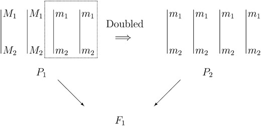
A pseudo-doubled backcross experiment for a tetraploid with two loci. Each locus is assumed to be biallelic: M1/m1 and M2/m2, where M1 and m1 denote two alleles of the first locus and M1 is the dominant allele, and similarly for M2 and m2. For each locus, there are two copies of the dominant allele in the informative parent P1. P2 is the noninformative doubled haploid produced by doubling a haploid of P1, which contains only recessive alleles.
, where an informative parent P1 is crossed with a noninformative parent P2. The dosage at each locus in the parents is at least one for the informative parent and zero for the noninformative parent. Furthermore, at most half of the chromosomes of the informative parent contain dominant alleles. Chromosomes that contain dominant alleles in the informative parent are called informative chromosomes. The pseudo-doubled backcross design is equivalent to doubling the half of the noninformative chromosomes of the informative parent to produce the noninformative parent and then crossing them to get F1. An example of a pseudo-doubled backcross experiment for a tetraploid (k = 4) with two marker loci M1 and M2 is shown in Figure 1. In this case, the dosage for both markers is two in the informative parent. A pseudo-doubled backcross population can also be developed from diploids by choosing two homozygous parents carrying different alleles, doubling each of them to produce tetraploids, crossing them to produce an F1, and then crossing the F1 to the parent containing recessive alleles.
Interval mapping:
Consider two flanking markers, M1 and M2, and one QTL, Q, with marker genetic distance or recombination fraction provided by an available genetic map. Once the parental configuration c is known, interval mapping can be applied to locate QTL. A parental configuration includes loci dosages and linkage phase. If the dominant alleles of two loci are on the same chromosome, they are in coupling phase; otherwise, they are in repulsion phase. On the basis of this, the five respective configurations for a tetraploid with two markers under a pseudo-doubled backcross design are called double coupling (Figure 2A)
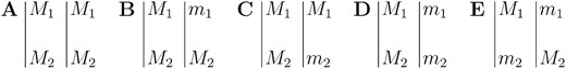
Possible parental marker configurations for a tetraploid with two marker loci (M1/m1 and M2/m2) under a pseudo-doubled backcross design. (A) Double coupling. (B) Asymmetric coupling 12. (C) Asymmetric coupling 21. (D) Coupling. (E) Repulsion.
, asymmetric coupling 12 (Figure 2B), asymmetric coupling 21 (Figure 2C), coupling (Figure 2D), and repulsion (Figure 2E). Similarly, there are three possible QTL configurations: (1) one dose of the QTL located on the first informative chromosome, (2) one dose of the QTL on the second informative chromosome, and (3) two doses of the QTL on both informative chromosomes. In what follows, configurations A–E are used to denote a marker configuration for a tetraploid as defined above. A marker configuration letter followed by a QTL configuration number represents a complete parental configuration, such as “A1,” which represents a parental configuration with markers in double coupling and one QTL on the first informative chromosome.
Since the estimation procedure is based on a specific parental configuration (model), the model space expands quickly as the marker number and/or ploidy level increase. Enumerating each possible model for the purpose of exploring which is most likely to produce the observed data and then estimating parameters on the basis of the most likely model(s) is computationally challenging. For example, under a pseudo-doubled backcross design with two markers and one QTL, there are 14 possible parental configurations for a tetraploid, 91 for a hexaploid (k = 6), and 390 for an octaploid (k = 8). To reduce these computations, we employ a model reduction step prior to parameter estimation.
Model reduction:
To reduce the model space, one can consider one of two approaches: either a marginal or a joint statistical method. Under the marginal method, we calculate the posterior probability of dosages for each marker individually. If one particular dosage level has a posterior probability higher than a specified cutoff, only that marker dosage is considered in candidate parental configurations. Otherwise, we select the most likely dosage levels until the sum of posterior probabilities exceeds the cutoff and these dosages are used to form the candidate parental configuration set. The joint method, on the other hand, takes a similar approach, but information on all markers is considered jointly. In this case, parental marker configuration posterior probabilities are calculated directly, and candidate parental configurations are chosen using the same posterior probability rule as described for the marginal method.
Multinomial distribution probability parameters
(M1M2|M1M2)a | (M1M2|M1) | (M1M2|M2) | (M1|M2) | (M2|M1) | |
|---|---|---|---|---|---|
| p00c | \(\frac{\mathit{r}^{2}\ {-}\ 2\mathit{r}\ +\ 1}{6}\) | \(\frac{1\ {-}\ \mathit{r}}{6}\) | \(\frac{1\ {-}\ \mathit{r}}{6}\) | \(\frac{1\ {-}\ \mathit{r}}{2}\) | \(\frac{1\ +\ \mathit{r}}{6}\) |
| p01c | \(\frac{{-}\mathit{r}^{2}\ +\ 2\mathit{r}}{6}\) | \(\frac{2\ +\ \mathit{r}}{6}\) | \(\frac{\mathit{r}}{6}\) | \(\frac{\mathit{r}}{2}\) | \(\frac{2\ {-}\ \mathit{r}}{6}\) |
| p10c | \(\frac{{-}\mathit{r}^{2}\ +\ 2\mathit{r}}{6}\) | \(\frac{\mathit{r}}{6}\) | \(\frac{2\ +\ \mathit{r}}{6}\) | \(\frac{\mathit{r}}{2}\) | \(\frac{2\ {-}\ \mathit{r}}{6}\) |
| p11c | \(\frac{\mathit{r}^{2}\ {-}\ 2\mathit{r}\ +\ 5}{6}\) | \(\frac{3\ {-}\ \mathit{r}}{6}\) | \(\frac{3\ {-}\ \mathit{r}}{6}\) | \(\frac{1\ {-}\ \mathit{r}}{2}\) | \(\frac{1\ +\ \mathit{r}}{6}\) |
Only dominant alleles are shown for informative chromosomes, separated by |.
r, estimated recombination fraction between the two markers.
Among the many criteria for assessing the worth of a model reduction method are ease of implementation, a high probability of selecting the correct model, and efficiency in reducing the size of the candidate model space. Even though the marginal method is easy to implement and less computationally expensive, the joint method directly estimates the posterior probability of parental marker configurations. One might expect that because there may be multiple marker configurations that have the same marker dosages, especially if the marker dosages are low and ploidy high, the joint method will be more efficient in reducing the model space.
A simulation study was performed to compare the performance of the marginal and joint methods for a tetraploid under random pairing. We chose two markers and marker genetic distance varied from 0.1 to 0.5 M with 0.1-M increments. Sample sizes ranged from 50 to 500 with increments of 50. For each simulation setting, 10,000 data sets were generated. The cutoff probability was set to be 0.90 for both methods. Without any prior information concerning the parental marker configuration, we assumed all the possible parental marker configurations to be equally likely (i.e., the prior for the joint method is discrete uniform). Under this assumption, the prior distribution of a marker dosage is not uniform since a lower dosage is more frequent than a higher dosage. Among the five possible parental marker configurations (Figure 2, A–E) for a tetraploid, dosage 1 has a frequency of 3/5 and dosage 2 has a frequency of 2/5 for each marker locus. In turn, this frequency distribution was used as the prior of marker dosage for the marginal method.
The proportion of data sets for which the correct configuration was included in the candidate configuration space, pinc, was recorded (Table 2)
Estimated pinc, probability of selecting the correct configuration in the candidate configuration (model) space, for a tetraploid with two markers, 10,000 simulated data sets, and a cutoff of 0.90 for both the marginal and joint model reduction methods under random pairing
n | |||||||||
|---|---|---|---|---|---|---|---|---|---|
| 50 | 100 | 150 | |||||||
| 0.1a | 0.3 | 0.5 | 0.1 | 0.3 | 0.5 | 0.1 | 0.3 | 0.5 | |
| Marginal | |||||||||
| (M1M2|M1M2) | 1.000 | 1.000 | 1.000 | 1.000 | 1.000 | 1.000 | 1.000 | 1.000 | 1.000 |
| (M1M2|m1M2) | 0.992 | 0.992 | 0.991 | 0.999 | 0.999 | 0.999 | 1.000 | 1.000 | 0.999 |
| (M1M2|M1m2) | 0.992 | 0.992 | 0.993 | 0.999 | 0.999 | 0.999 | 1.000 | 0.999 | 0.999 |
| (M1M2|m1m2) | 0.988 | 0.987 | 0.985 | 0.998 | 0.999 | 0.999 | 1.000 | 0.999 | 1.000 |
| (m1M2|M1m2) | 0.983 | 0.987 | 0.987 | 0.998 | 0.998 | 0.997 | 0.999 | 0.999 | 0.999 |
| Joint | |||||||||
| (M1M2|M1M2) | 0.999 | 0.999 | 0.999 | 1.000 | 1.000 | 1.000 | 1.000 | 1.000 | 1.000 |
| (M1M2|m1M2) | 0.999 | 0.999 | 0.998 | 1.000 | 1.000 | 1.000 | 1.000 | 1.000 | 1.000 |
| (M1M2|M1m2) | 1.000 | 0.999 | 0.998 | 1.000 | 1.000 | 0.999 | 1.000 | 1.000 | 1.000 |
| (M1M2|m1m2) | 0.999 | 0.998 | 0.988 | 1.000 | 1.000 | 0.999 | 1.000 | 1.000 | 0.999 |
| (m1M2|M1m2) | 0.999 | 0.999 | 0.992 | 1.000 | 0.999 | 0.999 | 1.000 | 1.000 | 0.999 |
Marker genetic distance expressed in morgans (M).
n, sample size.
for both methods. For the marginal method, this refers to selecting the correct marker dosages for both marker loci, while for the joint method it refers to selecting the correct marker configuration. The proportion of data sets for which a unique configuration was selected, puni, was also recorded as a measurement of the efficiency for reducing the model space (Table 3)
Estimated puni, probability of selecting a unique configuration in the candidate configuration (model) space, for a tetraploid with two markers, 10,000 simulated data sets, and a cutoff of 0.90 for both the marginal and joint model reduction methods under random pairing
n | |||||||||
|---|---|---|---|---|---|---|---|---|---|
| 50 | 100 | 150 | |||||||
| 0.1a | 0.3 | 0.5 | 0.1 | 0.3 | 0.5 | 0.1 | 0.3 | 0.5 | |
| Marginal | |||||||||
| (M1M2|M1M2) | 0.997 | 0.996 | 0.995 | 1.000 | 1.000 | 1.000 | 1.000 | 1.000 | 1.000 |
| (M1M2|m1M2) | 0.901 | 0.904 | 0.910 | 0.991 | 0.992 | 0.991 | 0.999 | 0.999 | 0.999 |
| (M1M2|M1m2) | 0.903 | 0.908 | 0.900 | 0.991 | 0.991 | 0.989 | 0.999 | 0.999 | 0.999 |
| (M1M2|m1m2) | 0.860 | 0.842 | 0.841 | 0.983 | 0.982 | 0.979 | 0.997 | 0.998 | 0.998 |
| (m1M2|M1m2) | 0.813 | 0.821 | 0.820 | 0.982 | 0.978 | 0.982 | 0.998 | 0.998 | 0.998 |
| Joint | |||||||||
| (M1M2|M1M2) | 0.992 | 0.989 | 0.983 | 0.999 | 1.000 | 0.999 | 1.000 | 1.000 | 0.999 |
| (M1M2|m1M2) | 0.999 | 0.991 | 0.979 | 1.000 | 0.999 | 0.999 | 1.000 | 1.000 | 1.000 |
| (M1M2|M1m2) | 0.999 | 0.989 | 0.978 | 1.000 | 1.000 | 0.999 | 1.000 | 1.000 | 1.000 |
| (M1M2|m1m2) | 0.991 | 0.981 | 0.867 | 0.999 | 0.999 | 0.981 | 1.000 | 1.000 | 0.997 |
| (m1M2|M1m2) | 0.999 | 0.987 | 0.900 | 1.000 | 0.999 | 0.985 | 1.000 | 1.000 | 0.997 |
Marker genetic distance expressed in morgans (M).
n, sample size.
. In general, both methods performed better with a larger sample size and shorter marker distances. With sample size ≥100, both pinc and puni were ∼1.0 for all the simulation settings. With a small sample size, the extra information from the genetic map added strength to the joint method both in selecting the correct configuration and in reducing the model space. On the basis of the simulation results, the joint model reduction method is recommended for data analysis.
Once the model reduction step is completed, the selected submodels are used to form the pool of candidate parental marker configurations by combining these submodels with possible parental QTL configurations. After this, the likelihood function is constructed for each candidate parental configuration, and the EM algorithm is applied to maximize the likelihood function and estimate parameters. The parental configuration that has the maximal likelihood is then identified as the parental configuration from which the observed data have arisen.
DATA ANALYSIS
The proposed approach was employed to analyze a published alfalfa SDRF data set with traits related to winter hardiness (Brouwer and Osborn 1999). Alfalfa is an autotetraploid that undergoes bivalent random pairing (Bingham and McCoy 1988; Cao et al. 2004). Winter hardiness is a complex trait and one of the most important adaptations for alfalfa. Because there is no direct measurement of winter hardiness, related traits including winter injury (WI), fall growth (FG), freezing injury (FI), and unifoliate internode length (UIL) were measured in addition to survival percentage of plants (SURV). SURV was measured by the percentage of each plant that survived in the winter (0–100%). FG was measured by height of vertical regrowth in centimeters in early October in two successive years, 1995 and 1996; FI was measured by absorbance at 265 nm (ABS) and electrical conductivity per gram fresh weight (COND) in 1995 and 1996; WI scaled 1–5 (1, no injury; 5, dead) was measured in 1996 and 1997; and UIL was measured for all seedlings. The histogram plots of these traits can be referred to Figure 1 in Brouwer et al. (2000).
Two genotypes, B17 and P13, representing the extremes for each trait were crossed, and a single F1 plant was crossed to each parent to create two populations of 101 individuals each. Both populations were scored for 82 SDRF loci and measured for each trait in 2 years of replicated field trials. The composite map and the original analysis of the trait data and marker data can be found in Brouwer and Osborn (1999) and Brouwer et al. (2000). On the basis of the genetic map, seven linkage groups were identified and corresponded to seven out of the eight chromosomes. As such in what follows, the terms for chromosome and linkage group are used interchangeably.
Because only B17 markers were considered for the P13 × F1 backcross population and similarly only P13 markers for the B17 × F1 backcross, each backcross population is equivalent to a pseudo-doubled backcross population. Our approach was applied to identify regions in the genome related to the previously described quantitative traits for both backcross populations based on the composite map. The average over the replicates in each year for each measurement was treated as a quantitative trait, and the two averages were analyzed separately. A permutation test (Churchill and Doerge 1994) with 1000 permutations for a 0.05 significance level was used to detect a significant QTL.
Seven QTL were detected for FG, two for FI, one for SURV, and one for WI in the backcross to B17; and one QTL was detected for UIL in the backcross to P13 (Table 4)
Estimated locations and effects of QTL associated with winter hardiness and its related traits for autotetraploid alfalfa
Trait | Year | Chr | Marker interval | Pos | d̂1 | dQ | μ̂a | σ̂ |
|---|---|---|---|---|---|---|---|---|
| FGb | 1995 | 1 | uwg284–vg2b9 | 0.31 | 0.31 | 2 | 12.24, 21.45, 24.61 | 2.61 |
| 1996 | 1 | uwg284–vg2b9 | 0.34 | 0.34 | 2 | 12.51, 19.18, 19.29 | 3.17 | |
| 1995 | 5 | vg2a2–vg2e5 | 0.498 | 0.001 | 2 | 12.30, 21.65, 23.75 | 2.82 | |
| 1996 | 5 | hg2b12–vg2a2 | 0.456 | 0.05 | 2 | 12.70, 18.48, 22.08 | 2.96 | |
| 1996 | 5 | mtsc35–ugac473 | 0.29 | 0.02 | 2 | 15.23, 18.46, 20.90 | 3.63 | |
| 1996 | 8 | ugac291–ugac540 | 0.187 | 0.10 | 2 | 13.02, 18.60, 21.53 | 3.08 | |
| 1996 | 8 | ugac109–uwg169 | 0.704 | 0.06 | 2 | 15.57, 18.95, 19.95 | 3.62 | |
| CONDc | 1996 | 6 | ugac281–vg2c2 | 0.356 | 0.09 | 2 | 52.42, 59.05, 94.60 | 13.30 |
| 1996 | 8 | ugc291–ugac540 | 0.247 | 0.16 | 2 | 50.91, 58.36, 92.89 | 12.64 | |
| SURVd | 1995 | 8 | ugac291–ugac540 | 0.187 | 0.10 | 1 | 0.54, 0.14 | 0.229 |
| WIe | 1996 | 8 | ugc291–ugac540 | 0.217 | 0.13 | 2 | 2.66, 4.40, 4.82 | 0.513 |
| UIL | — | 8 | ugac235–ugac291 | 0.001 | 0.001 | 2 | 9.34, 3.35, 12.74 | 1.847 |
μ = (μ0, μ1, … , μdQ) is the estimated mean vector.
The trait fall growth (FG) was measured by height of vertical regrowth in centimeters in early October in 2 successive years, 1995 and 1996.
Electrical conductivity per gram fresh weight (COND) was measured in 1995 and 1996 to represent freezing injury (FI).
Winter survival percentage of plants (SURV) was measured in 1995 and 1996 to represent winter hardiness.
Winter injury (WI) was scaled 1–5 (1, no injury; 5, dead) and was measured in 1996 and 1997.
Data are from Brouwer and Osborn (1999). Significant QTL were detected by experiment-wise thresholds calculated from 1000 permutation tests at the 0.05 significance level. Chr, chromosome number; Pos, estimated composite map position of the QTL; d̂1, genetic distance between the detected QTL and left end marker of the interval; dQ, estimated QTL dosage; σ, estimated common standard deviation of the trait. UIL, unifoliate internode length.
. Among the seven QTL detected for FG, two were mapped on chromosome 1, three on chromosome 5, and two on chromosome 8. Two pairs of QTL were detected at close map positions across 2 years: on chromosome 1, one QTL was detected at 0.31 M for the 1995 average and one at 0.34 M for the 1996 average; on chromosome 5, one QTL was detected at 0.498 M for the 1995 average and one at 0.456 M for the 1996 average. Two QTL were detected on chromosomes 6 and 8 for freezing injury FI. One QTL was detected on chromosome 8 for SURV and WI. On chromosome 8, in the region from 0.187 to 0.247 M, four QTL were detected for multiple traits, fall growth (FG 1996), freezing injury (COND 1996), winter hardiness (SURV 1995), and winter injury (1996); and two of them were at the same location, 0.187 M. The one QTL for UIL in the P13 backcross was at the top of chromosome 8. All of the detected QTL were identified to have dosage two, except for the QTL for winter hardiness (SURV). In general, an additional copy of a QTL was found to be associated with a higher quantitative trait mean, except for the QTL for SURV and UIL.
Brouwer et al. (2000) used a regression-based single-marker analysis to identify markers associated with the previously described quantitative traits. Multiple regression analyses were performed using the same data for all 82 SDRFs to identify the best polygenic models for each trait in each backcross population. With the backcross to B17, the SDRF multiple regression models include six SDRFs for FG (1995), six for FG (1996), five for FI (COND 1996), and four for WI (1996) [Table 5
Estimated locations of QTL affecting traits related to winter hardiness in Brouwer et al. (2000): (A) fall growth (FG) 1995 average; (B) fall growth (FG) 1996 average; (C) freezing injury (FI: COND) 1996 average; (D) winter injury (WI) 1996 average
A | B | C | D | ||||||||
|---|---|---|---|---|---|---|---|---|---|---|---|
| Chr | Marker | Pos | Chr | Marker | Pos | Chr | Marker | Pos | Chr | Marker | Pos |
| 1 | vg2b9 | 35.8a | 1 | vg2b9 | 35.8a | 1 | vg2b9 | 35.8b | 2 | vg0c5 | 23.0c |
| 1 | mtsc9 | 51.4 | 3 | mtsc14 | 46.1b | 1 | mtsc9 | 51.4d | 4 | ugac671 | 15.3 |
| 3 | uwg96 | 24.3b | 5 | mtsc35b | 27.0a | 3 | ugac224 | 23.1d | 8 | ugac540 | 30.9d |
| 3 | mtsc14 | 46.1c | 5 | ugac473 | 29.3a | 8 | ugac540 | 30.9c | 8 | ugac191 | 63.7 |
| 5 | vg2a2 | 49.8a | 8 | ugac540 | 30.9c | 8 | ugac191 | 63.7 | |||
| 8 | ugac191 | 63.7 | 8 | ugac191 | 63.7c | ||||||
Locus close to the QTL identified by the interval-mapping method.
LRT at this locus is a peak close to the 0.05 threshold.
LRT at this locus is higher than the 0.05 threshold, but not a peak.
LRT at this locus is a peak, not close to the 0.05 threshold.
Chr, chromosome; Pos, estimated composite map position of the QTL.
, summarized from Brouwer et al.'s (2000) Table 2]. Among all the detected SDRFs, all but five are located on chromosomes 1, 5, and 8, which also contain most of QTL we detected with the proposed method. Two loci for FG (1995) and three for FG (1996) are also shared by our interval-mapping method. Among the other significant marker loci, four had likelihood-ratio test statistics larger than the 0.05 experiment-wise threshold used in our interval-mapping method, but were not local peaks. Five loci had likelihood-ratio test statistics being local peaks, with two of them close to the 0.05 threshold.
Using an experiment-wise threshold based on a significance level 0.05, rather than an asymptotic-based strict cutoff based on a significance level 0.05 or 0.005 for each marker (Brouwer et al. 2000), we detected fewer QTL by controlling the type I error. The region on chromosome 8 (from 0.187 to 0.247 M) that was identified by our method as being shared by multiple traits was not detected by the regression method. This is most likely the direct result of more experimental information being incorporated into the analysis (e.g., model selection, dosages, intermarker position). Since single-marker analysis explores only the relationship between the quantitative trait and marker loci, if the QTL is very close to a marker locus, the estimated effect for that marker locus could be interpreted as the effect of the QTL, under the assumption that the QTL is also of a single dose and in coupling with the marker. However, most of the QTL that were detected using our method were of dosage two; therefore, it is not appropriate to compare the QTL effects estimated by Brouwer et al. (2000) with our method.
Ma et al. (2002) analyzed the same alfalfa data for two traits, WI and fall injury (FI: COND). They identified five QTL for FI: COND on chromosomes 4, 5, 6, and 8, and four QTL for winter injury on chromosomes 1, 5, and 8. The specifics of the Ma et al. (2002) method and analysis make a direct comparison between our results and their results difficult for the following reasons. First, it is assumed in Ma et al. (2002) that the markers and QTL have the same dosage level and are in coupling, while most of our detected QTL were of dosage two. Second, there is some evidence that the preferential pairing factor estimation process provided by Ma et al. (2002) is flawed since in reality the genotypic information collected for across years should not change, yet their estimates of preferential factor do (Cao et al. 2004). Finally, in Ma et al. (2002) the critical value for the significance level 5% is calculated on the basis of 200 permutation tests. For a 5% significance level (Churchill and Doerge 1994; Doerge and Churchill 1996), 200 permutations limit full exploration of the null space and may lead to the declaration of some QTL that are actually not significant at the 5% level.
SIMULATION
We used the framework provided by both the alfalfa experiment and analysis as a means to investigate the reliability of the detected QTL via a simulation study. Data were simulated by treating the estimated parental configuration and related parameters as the true values. For this purpose, 5 of the 12 QTL that we detected were chosen to provide a range for the flanking marker genetic distance and configuration, QTL dosage and configuration, QTL effect, and QTL position (Table 6)
Estimated QTL location and effect for data simulated from five intervals containing detected QTL as indicated by alfalfa data and analysis
QTL | Trait | Pos | Mconfig | Freq | d(M1, M2) | d1 | d̅̂1 \(\left(\mathit{s}\left(\mathit{{\hat{d}}}_{1}\right)\right)\) | σ | σ̅̂ | μa | μ̅̂ |
|---|---|---|---|---|---|---|---|---|---|---|---|
| 1 | FG | 0.31 | E | 999 | 0.358 | 0.31 | 0.30(0.066) | 2.61 | 2.55 | 12.24, 21.45, 24.61 | 12.32, 21.49, 24.54 |
| 2 | FG | 0.34 | E | 992 | 0.358 | 0.34 | 0.30(0.092) | 3.17 | 3.04 | 12.51, 19.18, 19.29 | 12.53, 19.21, 19.29 |
| 3 | FG | 0.456 | D | 862 | 0.098 | 0.05 | 0.059(0.036) | 2.96 | 2.82 | 12.70, 18.48, 22.08 | 12.68, 18.58, 21.89 |
| 4 | SURV | 0.187 | D | 955 | 0.222 | 0.10 | 0.097(0.041) | 0.23 | 0.23 | 0.54, 0.14 | 0.54, 0.14 |
| 5 | UIL | 0.001 | D | 954 | 0.087 | 0.001 | 0.015(0.027) | 1.85 | 1.86 | 9.34, 3.35, 12.74 | 9.14, 3.41, 12.50 |
μ = (μ0, μ1, … , μdQ) is the mean vector of the trait corresponding to QTL dosages.
For each interval, 1000 data sets of sample size 100 were simulated. Pos, position of the detected QTL on the composite genetic map; Mconfig, marker configuration (D is coupling and E is repulsion); d1, distance between the QTL and the left end marker; σ, common standard deviation of the trait for all QTL dosage levels; Freq, frequency of selecting the correct parental configuration out of 1000 data sets; d̅̂1, average of the 1000 estimated QTL locations from the 1000 simulated data sets; s
. The flanking marker distances were 0.358, 0.358, 0.098, 0.222, and 0.087 M for the five intervals (Table 6). The flanking markers in the first two intervals were in repulsion, and the others were in coupling. The estimated QTL dosage was one for the fourth interval and two for the other intervals. The simulation setting of the second interval was similar to that of the first interval. We included the second interval in our simulation because we were interested in investigating whether our method is able to identify the small increment from μ1 to μ2, where μ = (μ0, μ1, μ2) = (12.51, 19.18, 19.29) is the estimated mean vector for the corresponding QTL in that interval.
The five interval settings were studied separately. For each interval, 1000 data sets with a sample size of 100 (i.e., similar to the alfalfa data) were simulated and analyzed, with results summarized in Table 6. Using the joint model selection method, the correct parental marker configuration was included in the candidate parental marker configuration pool 100% of the time for all five cases. The overall parental configuration pool is then formed by the combination of candidate parental marker configurations and possible QTL configurations. After fitting our interval-mapping model to each possible parental configuration, the one having the maximal test statistic provides the estimated QTL location and marker and QTL configuration, as well as the parameter estimates. The correct configuration was identified at least 95% of the time with markers in coupling and at least 99% of the time with markers in repulsion, except for the third interval where the correct configuration was selected 86% of the time. Given the correct configuration, the estimated parameters were close to the true values used for simulation.
The fact that our method performed better with repulsion than with coupling is due to the difference between these two configurations. This can be demonstrated by considering an example where two copies of the QTL are on both informative chromosomes. When the markers are in coupling, one copy of the QTL is located on a chromosome containing no dominant marker alleles. Thus, not much extra information with respect to the recombination between markers and the QTL can be provided by this extra copy of the QTL. This, in turn, makes it difficult to choose between the configurations with one copy and two copies of the QTL. On the other hand, with markers in repulsion, both copies of the QTL provide information about recombination between markers and QTL. The effect of this difference is easily illustrated by comparing the second interval with the third interval used for this simulation. Although the increment in trait means from QTL dose 1 to dose 2 is only 0.035σ for case 2 and 1.22σ for case 3, case 2 still outperformed case 3. On the basis of this, repulsion is not necessarily the worst-case scenario for QTL mapping in tetraploids with simplex markers, as was once thought.
Since the above simulation was mainly focused on parental marker configurations formed by simplex markers, another simulation study was performed to serve as the basis of investigation for how, in general, QTL or marker dosages and their respective linkage phase affect the performance of our algorithm. Under a pseudo-doubled backcross experiment, two markers (M1/m1 and M2/m2) and one QTL (Q/q) were used with marker distance 0.10 M and a sample size 100. The location of the QTL was 0.01, 0.03, or 0.05 M. The trait mean μ was (10.0, 12.0) if QTL dosage was 1 or (10.0, 12.0, 14.0) if QTL dosage was 2, and σ was 1.0. One thousand data sets were simulated for each combination of the parameter settings and each of the following configurations: double coupling (A1, A3), asymmetric coupling 12 (B1, B2, B3), coupling (D1, D2, D3), and repulsion (E1, E2, E3).
Our simulation results illustrate that when the correct parental configuration was identified, the parameter estimate averages were close to the true value. The ability to identify the correct configuration, however, depended on the underlying parental configuration. The worst-case scenario was when markers were in coupling on the first informative chromosome with one copy of the QTL on the second informative chromosome (D2). For this case the identified correct configuration proportion ranged from 63 to 66% (Figure 3)
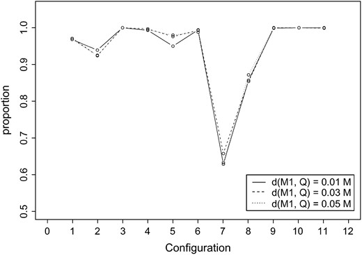
The proportion identifying the correct parental (marker and QTL) configuration for a tetraploid under a pseudo-doubled backcross experiment. The trait mean μ is (10.0, 12.0) if QTL dosage is 1 or (10.0, 12.0, 14.0) if QTL dosage is 2. Population standard deviation σ is 1.0. With sample size 100, 1000 data sets are simulated under 11 parental configurations corresponding to numbers 1–11 on the horizontal axis: A1, A3, B1, B2, B3, D1, D2, D3, E1, E2, and E3. The letters denote the marker configurations: (A) double coupling, (B) asymmetric coupling 12, (D) coupling, and (E) repulsion. The numbers denote the QTL configurations: (1) one dose of QTL present on the first informative chromosome, (2) one dose of QTL present on the second informative chromosome, and (3) two doses of QTL present on both informative chromosomes. d(M1, Q) is the genetic distance between the QTL and the left end-flanking marker.
. This is not surprising since with D2 under random pairing, only one-third of the pairings provide information concerning the recombination between marker and QTL. On the other hand, the best situation was when two markers were in repulsion, where the correct parental configuration was almost 100% regardless of the QTL configuration or location. Most of the other configurations obtained a proportion of at least 95% (Figure 3).
It is worth noting that in our earlier work (Cao et al. 2003), repulsion did not outperform configurations with higher dosages of loci, such as double coupling and asymmetric coupling. The difference in results comes from the difference in the assumed chromosome-pairing mechanism. Our earlier work (Cao et al. 2003) investigated the performance of our interval-mapping method under preferential pairing, which specifically deals with bivalent pairing (i.e., an informative chromosome pairs only with a noninformative chromosome). The preferential pairing mechanism is favorable to configurations with higher dosages of loci because it maximizes the amount of recombination information through maximizing the disequilibrium in pairing. However, with random pairing, one-third of the time one informative chromosome pairs with another informative chromosome to provide less, or even no, information, if two chromosomes are homozygous. Using similar reasoning it can be demonstrated that random pairing is more informative than preferential pairing for markers in repulsion.
DISCUSSION
One of the largest challenges when mapping QTL in polyploids is the incomplete parental configuration (model) information. This is compounded by the dramatic increase in the size of the model space as the number of markers and/or ploidy level increase. To combat these challenges in autopolyploid QTL mapping, our interval-mapping algorithm takes one of two approaches. The size of the model space is addressed using Bayesian model selection by first identifying potential parental marker dosages using a marginal approach or marker configurations based on a joint approach. We have demonstrated that both methods are effective in reducing the model space, but that the joint method is more efficient due to the fact that it incorporates the genetic map information. From the reduced model space, the candidate parental configuration pool is formed by combining each potential parental marker configuration with a possible QTL configuration. For each potential parental configuration, profiles of MLEs of QTL effects, as well as population variation and likelihood-ratio test statistics, are produced at each evaluation point of a grid search across the genome. Putative QTL are detected using a resampling-based significance threshold. The corresponding parental configuration (and related parameter estimates) is then taken as the underlying model from which the data are produced.
Our simulation studies have demonstrated that if the correct parental configuration is identified, our interval-mapping method provides parameter estimates close to true values. However, the chance of identifying the correct configuration depends on the true parental configuration, chromosome pairing system, and genetic distance between markers and the QTL. This helps us address a question raised in Doerge and Craig (2000)(p. 7956), “for which situation is the linkage mostly affected?” Comparatively, among these factors, the true parental configuration is the most influential one. Since a configuration consists of both loci dosages and linkage phase, the influence of one cannot be considered without considering the effect of the other. For example, a configuration with higher marker/QTL dosages does not always imply a greater chance of identifying the correct configuration as shown in the case of repulsion. However, a configuration with higher dosages is often more informative because it often has a higher disequilibrium, which as we all know is the basis for linkage analysis. Furthermore, such a configuration is less sensitive to the chromosome-pairing system and thus consistently provides high power for detecting QTL.
Our simulation results also help to answer some of the remaining questions presented by Doerge and Craig (2000)(p. 7956). First, “If a molecular marker is found to be tightly linked to a QTL, should the dosage of the marker agree with the dosage of the QTL?” Not necessarily. There is no causal relationship between the dosages of the QTL and the flanking markers. Although as discussed previously a configuration with the marker and QTL having the same dosage often has a higher disequilibrium and thus a higher power of detecting QTL. Second, “Should the models which are controlled by dosage levels be weighted for the purpose of representing more realistic results?” Weighting the candidate models may be a better way than depending solely on the one “best” model, when the uncertainty about parental configuration is high. However, even configurations with the same marker dosage levels could differ to a greater extent biologically; therefore, further investigation is needed to find a both statistically and biologically sound weighting scheme. Finally, “Would models with dosage levels more similar to each other be more likely, especially with close linkage (short genetic distance)?” This answer depends on the linkage phase since it is possible for two models with exactly the same dosage levels and genetic association to be biologically different due to different linkage phases, and therefore they are different in likelihood.
We applied our approach to a published alfalfa data set for quantitative traits that are related to winter hardiness. Our analysis confirms several putative QTL identified by a regression-based single-marker analysis (Brouwer et al. 2000), and it also identified a new region on chromosome 8 that was shared by several traits. Our analysis results demonstrate that for a majority of the detected QTL, there is a positive or negative correlation between the quantitative trait mean and QTL dosage level; i.e., μ0 ≤ μ1 ≤ … ≤ μdQ or μ0 ≥ μ1 ≥ … ≥ μdQ. If such an ordering of means is available before analysis, an order-restricted version of interval mapping can be performed to improve power of detection. With an order constraint, the problem falls into the category of isotonic regression and it can be computed using the pool-adjacent-violator algorithm (Robertson et al. 1988). We have performed simulations (not shown) to compare the power between an order restriction and without one. In fact, even when the only information is that the means are ordered, and the direction remains unknown, there is a slight improvement in the performance. The improvement is most evident when the order of the means is increasing or decreasing with respect to the QTL dosage and is known a priori.
Thus far it has been assumed that the QTL dosage is at most half the ploidy level, which is a reasonable assumption given the pseudo-doubled backcross experimental design that we considered. In practice, if this assumption does not hold, we can simply change the upper bound for the QTL dosage to the ploidy level. This change will result in more candidate QTL configurations to choose from, but the method and the procedure remain the same. Similarly, if the breeding design is altered from a pseudo-doubled backcross design, our approach can be adapted. Also, if codominant markers are considered, they can be easily incorporated in the model by including parameters such as allelic effect and interaction.
The effect of the assumptions we place on the genetic map that is used for QTL mapping in polyploids is one area of research that remains unaddressed. When the genetic map is estimated, the most likely parental marker configuration in turn has to be estimated since recombination requires a parental marker configuration. Because of this, the parental marker configuration used for estimating the genetic map should be consistent with the one used to locate QTL. However, if the most likely parental marker configuration is not the correct configuration, the reliability of the map and the mapped QTL are affected. By selecting the pool of potential parental configurations on the basis of observed progeny data, our method can serve as a further verification for the estimated genetic map. A framework is currently under development to allow variability or uncertainty in estimating the map to be considered when mapping QTL.
Footnotes
Communicating editor: C. Haley
Acknowledgement
We thank Tom Osborn for providing the data set and continued work in this area, and we thank Gary Churchill for his comments on this work.
References
Bayes, T.,
Bingham, E. T., and T. J. McCoy, 1988 Cytology and cytogenetics of alfalfa, pp. 737–776 in Alfalfa and Alfalfa Improvement, edited by A. A. Hanson, D. K. Barnes and R. R. Hill, Jr. American Society of Agronomy, Madison, WI.
Broman, K. W.,
Brouwer, D., and T. Osborn,
Brouwer, D. J., S. H. Duke and T. C. Osborn,
Cao, D., B. A. Craig and R. W. Doerge, 2003 Interval mapping for autopolyploids, pp. 60–72 in Proceedings of the 15th Annual Kansas State University Conference on Applied Statistics in Agriculture, edited by G. Milliken. Kansas State University, Manhattan, KS.
Cao, D., T. C. Osborn and R. W. Doerge,
Churchill, G. A., and R. W. Doerge,
Darlington, C. D.,
Dempster, A. P., N. M. Laird and D. B. Rubin,
Dietrich, W. F., J. Miller, R. Steen, M. A. Merchant, D. Damron-Boles et al.,
Doerge, R. W.,
Doerge, R. W., and G. A. Churchill,
Doerge, R. W., and B. A. Craig,
Doerge, R. W., Z-B. Zeng and B. S. Weir,
Grattapaglia, D., and R. Sederoff,
Hackett, C. A., J. E. Bradshaw and J. W. McNicol,
Haley, C. S., and S. A. Knott,
Jackson, R. C., and J. W. Jackson,
Jansen, R. C.,
Knapp, S. J., J. W. C. Bridges and D. Brikes,
Koornneef, M., J. van Eden, C. J. Hanhart, P. Stam, F. J. Braaksma et al.,
Lander, E. S., and D. Botstein,
Luo, Z. W., C. A. Hackett, J. E. Bradshaw, J. W. McNicol and D. Milbourne,
Luo, Z. W., C. A. Hackett, J. E. Bradshaw, J. W. McNicol and D. Milbourne,
Luo, Z. W., R. Zhang and M. J. Kearsey,
Ma, C.-X., G. Casella, Z.-J. Shen, T. C. Osborn and R. Wu,
Muller, H. J.,
Osborn, T., J. Pires, J. Birchler, D. L. Auger, Z. J. Chen et al.,
Rieseberg, L. H., and M. F. Doyle,
Ripol, M., G. Churchill, J. da Silva and M. Sorrells,
Robertson, T., F. T. Wright and R. L. Dykstra, 1988 Order Restricted Statistical Inference, Ed. 1. Wiley, New York.
Rodzen, J. A., and B. May,
Soltis, D. E., and P. S. Soltis,
Soltis, D. E., P. E. Soltis and J. A. Tate,
Soltis, P. S., and D. E. Soltis,
Suzuki, D. T., A. J. F. Griffiths, J. H. Miller and R. C. Lewontin, 1989. Introduction to Genetics, Ed. 4. W. H. Freeman, New York.
Sybenga, J.,
Wolfe, K. H.,
Wu, K. K., W. Burnquist, M. Sorrells, T. L. Tew, P. H. Moore et al.,
Zeng, Z-B.,
