Predicting Genetic Values: A Kernel-Based Best Linear Unbiased Prediction With Genomic Data

Ober, Ulrike; Erbe, Malena; Long, Nanye; Porcu, Emilio; Schlather, Martin; Simianer, Henner

doi:10.1534/genetics.111.128694

Abstract

Genomic data provide a valuable source of information for modeling covariance structures, allowing a more accurate prediction of total genetic values (GVs). We apply the kriging concept, originally developed in the geostatistical context for predictions in the low-dimensional space, to the high-dimensional space spanned by genomic single nucleotide polymorphism (SNP) vectors and study its properties in different gene-action scenarios. Two different kriging methods [“universal kriging” (UK) and “simple kriging” (SK)] are presented. As a novelty, we suggest use of the family of Matérn covariance functions to model the covariance structure of SNP vectors. A genomic best linear unbiased prediction (GBLUP) is applied as a reference method. The three approaches are compared in a whole-genome simulation study considering additive, additive-dominance, and epistatic gene-action models. Predictive performance is measured in terms of correlation between true and predicted GVs and average true GVs of the individuals ranked best by prediction. We show that UK outperforms GBLUP in the presence of dominance and epistatic effects. In a limiting case, it is shown that the genomic covariance structure proposed by VanRaden (2008) can be considered as a covariance function with corresponding quadratic variogram. We also prove theoretically that if a specific linear relationship exists between covariance matrices for two linear mixed models, the GVs resulting from BLUP are linked by a scaling factor. Finally, the relation of kriging to other models is discussed and further options for modeling the covariance structure, which might be more appropriate in the genomic context, are suggested.

PREDICTING genotypes and phenotypes plays an important role in many areas of life sciences. Both in animal and plant breeding, it is essential to predict the genetic quality (the so-called total genetic value, GV) of individuals or lines, on the basis of different sources of knowledge. Often, phenotypic measures for various traits are available and the additive genetic relationship between individuals (Wright 1922) can be derived, on the basis of the known pedigree. Best linear unbiased prediction (BLUP; Henderson 1973) of breeding values is a well-established methodology in animal breeding (Mrode 2005) and has recently gained relevance in plant breeding (Piephoet al. 2008). In both areas, the main interest is in complex traits with a quantitative genetic background.

In human medicine, the interest is in predicting phenotypes, rather than genotypes, for simple or complex traits (e.g., the probability/risk to encounter a certain disease). Genetic prediction is mainly applied in the context of genetic counseling by predicting the risk of genetic disorders with known mono- or oligogenetic modes of inheritance and a certain history of cases in a known family structure, but accurate predictions of genetic predispositions to human diseases should also be useful for preventive and personalized medicine (delosCamposet al. 2010). Wrayet al. (2007) discuss the potential use of prediction of the genetic liability for traits with a complex quantitative genetic background in a human genetics context, and the variety of possible methods, including linear models, penalized estimation methods, and Bayesian approaches was reviewed by delosCamposet al. (2010).

With the availability of high-throughput genotyping facilities (Ranadeet al. 2001), genotypes for massive numbers of single nucleotide polymorphisms (SNPs) are available and can be used as an additional source of information for predicting GVs. Meuwissenet al. (2001) have suggested including SNP information in a statistical model of prediction. They used three statistical models: a model assigning random effects to all available SNPs (later termed “genomic BLUP”), assuming all SNP effects to be drawn from the same normal distribution, and two Bayesian models, where all (“Bayes A”) or a subset (“Bayes B”) of the random SNP effects are drawn from distributions with different variances. Various modifications of these methods and additional models have been subsequently suggested (Gianolaet al. 2009).

Gianolaet al. (2006) and Gianola and van Kaam (2008) have suggested a nonparametric treatment of genomic information by using reproducing kernel Hilbert spaces (RKHS) regression, which has already been demonstrated with real data (González-Recioet al. 2008, 2009). As was argued by delosCamposet al. (2009), the RKHS regression approach to genomic modeling represents a generalized class of estimators and provides a framework for genetic evaluation of quantitative traits that can be used to incorporate information on pedigrees, markers, or any other ways of characterizing the genetic background of individuals.

Opportunities to enhance genetic analyses by using nonparametric kernel-based statistical methods are enormous and these methods have been considered in different areas of genetic research. Schaid (2010a,b) provides an overview of measures of genomic similarity based on kernel methods and describes how kernel functions can be incorporated into different statistical methods like, e.g., nonparametric regression, support vector machines, or regularization in a mixed model context. Only recently, kernel-based methods have also been used in association studies (Kweeet al. 2008; Yanget al. 2008) and QTL mapping for complex traits (Zouet al. 2010), which demonstrates their great potential and flexibility.

Prediction is also relevant in other areas of research: In large parts of geostatistics, the spatial distribution of variables (like temperature, humidity, ore concentration, etc.) is considered. On the basis of a given (limited) set of measurements, the prediction of the variable realization in any point of the considered space is of interest. A standard approach for prediction in this case is the so-called “kriging” (Chilès and Delfiner 1999), which makes use of a parameterized covariance function of the regionalized variables.

While in geostatistics the application of kriging is naturally limited to few dimensions, the basic approach is rather universal (Schölkopfet al. 2004). In this article we apply kriging to the genomic prediction problem. Here, one dimension reflects genotype realizations at one SNP. In the genomic context, with p SNPs, realizations are in a p-dimensional orthogonal hypercube. Due to the biallelic nature of SNPs, only three genotype realizations (coded, e.g., as 0, 1, and 2) are possible in each dimension, so that the number of possible genotype constellations over p SNPs is 3^p.

The concept of kriging is closely related to the concept of BLUP. Cressie (1989) provides a “historical map of kriging” up to 1963 in which he also refers to Henderson (1963) who introduced BLUP in animal breeding. The steps of kriging are equivalent to “empirical BLUP”-procedures known in other frameworks, and kriging can be viewed as a “spatial BLUP.” The conceptual equivalence of geostatistical kriging and BLUP has already been discussed by Harville (1984). Robinson (1991) provides a detailed review of the history of estimation of random effects via BLUP and its various derivations. He also points out the similarities between BLUP and kriging.

The equivalence of kriging with BLUP in a space spanned by genomic data was first noted by Piepho (2009), who also discusses relationships with other estimation principles, like ridge regression (Whittakeret al. 2000) and least squares support vector machines (Suykenset al. 2002). Comparing the performance of spatial mixed models to ridge regression with maize data, he found that spatial models provide an attractive alternative for prediction. He also points out that the BLUP model used in Meuwissenet al. (2001) has an interpretation as a spatial model with quadratic covariance function. Spatial models for genomic prediction were also used by Schulz-Streeck and Piepho (2010).

Moreover, kriging is known to be closely related to radial basis function (RBF) regression methods (Myers 1992). Longet al. (2010) showed with real and simulated data that nonparametric RBF regression methods can outperform Bayes A when predicting total GVs in the presence of nonadditive effects using SNP markers.

In this article we demonstrate the potential of the kriging approaches applied to genomic data: As a novelty, we suggest the family of Matérn covariance functions to reflect the functional dependency of the observed covariances from the distance of genotypes expressed as Euclidean norm. On the basis of this model and the assumed covariance function, we suggest two kriging approaches. Under both models, parameters and hidden variables are estimated via maximum likelihood (ML) and BLUP of the unknowns is established by solving the corresponding linear kriging systems. All predictions can also be implemented in the form of the so-called mixed model equations (Henderson 1973). The predictive performance of the two models is compared to a common genomic BLUP as a reference method in a whole-genome simulation study considering various gene-action models.

Furthermore, we show that in a limiting case the genomic covariance structure proposed by VanRaden (2008) can be considered as a covariance function with corresponding quadratic variogram. In addition we prove theoretically that predicted GVs are scaled only by a factor if the covariance structures are linearly transformed. Finally, we discuss further options for a more differentiated modeling using the suggested methodological approach.

Methods

Kriging

The term kriging stems from the prediction of ore concentrations in deposits and was mainly developed by Matheron (1962, 1963) on the basis of the master’s thesis of Krige (1951). In geostatistics, kriging is currently the standard approach whenever spatial prediction of a so-called regionalized variable (Matheron 1989), e.g., temperature, ozone concentration or soil moisture, must be performed on the basis of a few isolated measurements of the quantity. It is assumed that the regionalized variable is a realization of a random function with a certain covariance structure. Mostly, the latter is given by a parameterized covariance function (Cressie 1993), and the random function is assumed to be Gaussian.

The kriging approach consists of two steps: (i) estimation of the unknown parameters and hidden variables (in particular by ML or REML) and (ii) prediction of the values of the regionalized variables by performing a BLUP, under the auxiliary assumption that the parameter values and hidden variables estimated in the first step are the true ones.

Many variants of the general kriging principle have been discussed (Cressie 1993). The type of kriging is implied by the unbiasedness condition: In “simple kriging” (SK), it is assumed that the underlying regionalized variable has zero mean, whereas in “universal kriging” (UK), a linear model for the mean of the underlying regionalized variable is assumed.

The model for polygenic and genomic data

In our further studies, we assume to have q individuals with pedigree information, n of them being genotyped and having phenotype measurements of a certain quantitative trait. Typically, GVs have to be predicted for individuals that are genotyped, but have no phenotype data.

We use the following model for the given data

y_{i} = w_{i}^{T} β + z_{i}^{T} u + g (x_{i}) + e_{i}, i = 1, \dots n,

where y_i is a measurement of the phenotype for individual i, β is an f-vector of nuisance location parameters, x_i is a p-vector of dummy SNP instance variates (genotype) observed on individual i, and g is an unknown, random function as described below. Let

u \sim N (0, σ_{u}^{2} A)

be a q-vector of additive genetic effects of q individuals, where

σ_{u}^{2}

is the additive genetic variance due to unmarked polygenes, and A is the numerator relationship matrix. The entries of the numerator relationship matrix are twice the coefficients of coancestry between individuals. The vectors

w_{i}^{T}

and

z_{i}^{T}

are known incidence vectors; z_i is a unit vector with one component being 1 and all the others zero, indicating the respective position in the pedigree. Let e = (e₁,…, e_n)^T be the vector of environmental residual effects with

e \sim N (0, σ_{e}^{2} I),

where

σ_{e}^{2}

is the environmental variance.

We assume that {g(x_i), x_i ε $ℝ^{p}$ } is a Gaussian random field (Lifshits 1995) with $E$ (g(x_i)) = 0 and covariance structure given by $Cov (g (x_{i}), g (x_{j})) = E (g (x_{i}) g (x_{j})) = K_{ν, h, σ_{K}} (x_{i}, x_{j}),$ where $K_{ν, h, σ_{K}} (\cdot, \cdot)$ is a covariance function depending on parameters ν, h, and σ_K_. Let $K_{ν, h, σ_{K}} = {(K_{ν, h, σ_{K}} (x_{i}, x_{j}))}_{1 \leq i, j \leq n}$ be the corresponding covariance matrix.

The family of Matérn covariance functions

For the covariance structure we suggest using the so-called family of Matérn covariance functions, which was introduced by Matérn (1986) and Handcock and Wallis (1994) and is defined by

Cov (g (x_{i}), g (x_{j})) = K_{ν, h, σ_{K}} (x_{i}, x_{j}) = σ_{K}^{2} \cdot \frac{2^{1 - ν}}{Γ (ν)} {(\sqrt{2 ν} ‖ x_{i} - x_{j} ‖ / h)}^{ν} K_{ν} (\sqrt{2 ν} ‖ x_{i} - x_{j} ‖ / h) .

Here, ‖ · ‖ is the Euclidean norm, ν > 0 is a smoothness parameter, h is a scale parameter,

σ_{K}^{2}

is the variance parameter, and

K_{ν} (\cdot)

is a modified Bessel function of the second kind of order ν (Abramowitz and Stegun 1984). The Matérn function is isotropic, in that Cov(g(x_i), g(x_j)) depends only on the Euclidean norm of the separation vector x_i – x_j.

Matérn covariance functions build a very general class of covariance functions including special cases like the exponential (ν = $\frac{1}{2}$ ⁠) and the Gaussian (ν = ∞) covariance function, the ones that have also been used by Piepho (2009). If the smoothness parameter ν is of the form m + $\frac{1}{2}$ ⁠, where m is an integer, the Matérn function factorizes into the product of an exponential function and a polynomial of degree m; cf.Table 1 and Figure 1. The best fitting parameter value ν is determined through the model-fitting approaches described below.

TABLE 1

Special cases of Matérn covariance functions

	ν	h	$K_{ν, h, σ_{K}} (x_{i}, x_{j})$
Exponential	0.5	1	$σ_{K}^{2} \cdot \exp (- \| \| x_{i} - x_{j} \| \|)$
	1.5	1	$σ_{K}^{2} \cdot \exp (- \sqrt{3} \| \| x_{i} - x_{j} \| \|) \cdot (1 + \sqrt{3} \| \| x_{i} - x_{j} \| \|)$
	2.5	1	$σ_{K}^{2} \cdot \exp (- \sqrt{5} \| \| x_{i} - x_{j} \| \|) \cdot (1 + \sqrt{5} \| \| x_{i} - x_{j} \| \| + \frac{5}{3} \| \| x_{i} - x_{j} \| \|^{2})$
Gaussian	∞	1	$\exp (- \frac{1}{2} \| \| x_{i} - x_{j} \| \|^{2})$

Open in new tab

Figure 1.—

Open in new tab Download slide

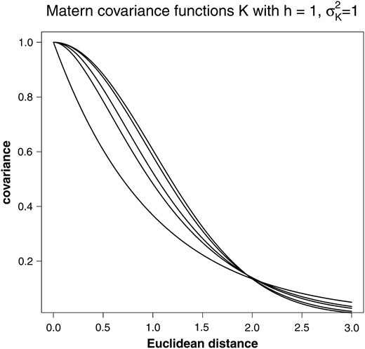
Matérn covariance functions for h = 1, $σ_{K}^{2} = 1$ ⁠, and different values of ν. From top to bottom ν = ∞, 10, 2.5, 1.5, 0.5.

In matrix notation, the statistical model is

y = W β + Zu + g (X) + e,

(1)

where

W = {(w_{1}^{T}, \dots, w_{n}^{T})}^{T}

is an (n × f)- and

Z = {(z_{1}^{T}, \dots, z_{n}^{T})}^{T}

is an (n × q)-incidence matrix and g(X) = (g(x₁),…, g(x_n))^T. Finally, we assume that the random vectors u, e, and g(X) are independent.

Two kriging approaches and a reference model

We consider two models to predict the total genetic value $z_{0}^{T} u + g (x_{0})$ of a certain genotyped individual indexed by 0. This individual belongs to the set of q individuals, but it does not have to be phenotyped. The models differ in the size of the sets of quantities that are estimated in the first kriging step and subsequently used for predictions.

Universal kriging: Modeling of y

We exploit the fact that y has a multivariate normal distribution,

y \sim N (W β, σ_{u}^{2} Z A {AZ}^{T} + K_{ν, h, σ_{K}} + σ_{e}^{2} I),

and estimate the parameters β, σ_u, σ_e, ν, h and σ_K by maximizing the log likelihood of the corresponding density function.

Then, we perform a best linear unbiased prediction of g(x₀) and

z_{0}^{T} u;

i.e., we apply the BLUP principle: To obtain

\hat{g} (x_{0})

we minimize

E {(\hat{g} (x_{0}) - g (x_{0}))}^{2} \to \min!

with the linear predictor

\hat{g} (x_{0}) = a_{g}^{T} y

under the condition

a_{g}^{T} W = 0.

This approach is called universal kriging in other areas of research (Cressie 1993). In fact, the condition assures

a_{g}^{T} W β = 0

and therefore

E g (x_{0}) = 0 = a_{g}^{T} W β = E \hat{g} (x_{0}),

i.e.,

\hat{g} (x_{0})

is unbiased. Let

K_{0} = {(K_{ν, h, σ_{K}} (x_{1}, x_{0}), \dots, K_{ν, h, σ_{K}} (x_{n}, x_{0}))}^{T} .

The approach results in the following kriging system of equations:

[\begin{matrix} W & σ_{u}^{2} Z A {AZ}^{T} + K_{ν, h, σ_{K}} + σ_{e}^{2} I \\ 0 & W^{T} \end{matrix}] \cdot [\begin{matrix} λ \\ a_{g} \end{matrix}] = [\begin{matrix} K_{0} \\ 0 \end{matrix}] .

Note that this linear system does not depend on β. Analogously,

z_{0}^{T} u

can be predicted by the universal kriging estimator

\hat{z_{0}^{T} u} = a_{u}^{T} y,

where a_u satisfies

[\begin{matrix} W & σ_{u}^{2} ZA Z^{T} + K_{ν, h, σ_{K}} + σ_{e}^{2} I \\ 0 & W^{T} \end{matrix}] \cdot [\begin{matrix} λ \\ a_{u} \end{matrix}] = [\begin{matrix} σ_{u}^{2} ZA z_{0} \\ 0 \end{matrix}] .

and one gets

\hat{z_{0}^{T} u} + \hat{g} (x_{0})

as BLUP of

z_{0}^{T} u + g (x_{0}) .

In the animal breeding context it is well known that a BLUP approach for the model y = Wβ + Zu + g(X) + e is equivalent to solving the mixed model equations (MME)

[\begin{matrix} W^{T} W & W^{T} Z & W^{T} \\ Z^{T} W & Z^{T} Z + \frac{σ_{e}^{2}}{σ_{u}^{2}} A^{- 1} & Z^{T} \\ W & Z & I + σ_{e}^{2} K_{ν, h, σ_{K}}^{- 1} \end{matrix}] \cdot [\begin{matrix} \hat{β} \\ \hat{u} \\ \tilde{α} \end{matrix}] = [\begin{matrix} W^{T} y \\ Z^{T} y \\ y \end{matrix}]

(2)

for given variance components estimated, e.g., by ML. For a derivation of the MME from the kriging system see, e.g.,Dempfle (1982).

Simple Kriging: Joint modeling of y, u, and g(X)

In the second approach we model the hidden variables u and g(X) explicitly and consider the joint density function f_y,u,g of y, u, and g(X), which equals

\begin{matrix} f_{y, u, g (X)} (y, u, g (X)) = f_{y | u, g (X)} (y) \cdot f_{u} (u) \cdot f_{g} (g (X)) \\ = f_{e} (y - W β - Zu - g (X)) \cdot f_{u} (u) \cdot f_{g} (g (X)) \\ = c \cdot \exp (- \frac{1}{2} \cdot [\frac{1}{σ_{e}^{2}} | | y - W β - Zu - g (X) | |^{2}]) \\ \cdot \exp (- \frac{1}{2} \cdot [\frac{1}{σ_{u}^{2}} u^{T} A^{- 1} u]) \cdot \exp (- \frac{1}{2} \cdot [g {(X)}^{T} K_{ν, h, σ_{K}}^{- 1} g (X)]) \end{matrix}

with

c^{- 1} = {(2 π)}^{n + q / 2} σ_{e}^{n} \cdot σ_{u}^{q} {(\det A)}^{1 / 2} \cdot {(\det K_{ν, h, σ_{K}})}^{1 / 2} .

Here, we have to estimate the parameters β, σ_u, σ_e, ν, h, σ_K and the hidden variables u and g(X). Note that in this approach we consider u and g(X) to be parameters that have to be estimated via ML in the first kriging step. Therefore, we maximize the log likelihood J of the density function f_y_,u,g; i.e., we maximize

J = \log (c) - \frac{1}{2} \cdot [\frac{1}{σ_{e}^{2}} | | y - W β - Zu u - g (X) | |^{2} + \frac{1}{σ_{u}^{2}} u^{T} A^{- 1} u + g {(X)}^{T} K_{ν, h, σ_{K}}^{- 1} g (X)],

(3)

with respect to β, u, and g(X). Taking the derivatives with respect to β, u, and g(X) leads to the linear system given in (2), which yields estimators for β, u, and g(X). When using these estimates in Equation 3, the value of J depends only on σ_u, σ_e, ν, h, and σ_K_. Thus, J can be maximized numerically with respect to these parameters, leading to estimates for β, σ_u, σ_e, ν, h, σ_K, u, and g(X). According to the kriging philosophy, we now assume the values of the estimators (especially the value of the estimator for g(X)) to be the true ones, and g(x₀) is predicted via

\hat{g} (x_{0}) = a_{g}^{T} g (X)

by the BLUP principle. That is, we minimize

E {(\hat{g} (x_{0}) - g (x_{0}))}^{2} \to \min!

with the linear estimator

\hat{g} (x_{0}) = a_{g}^{T} g (X) .

This approach is called simple kriging (Cressie 1989, 1993; Chilès and Delfiner, 1999). Note that

\hat{g} (x_{0})

is always unbiased. The solution is

\hat{g} (x_{0}) = K_{0}^{T} K_{ν, h, σ_{K}}^{- 1} g (X) .

(4)

Finally, the predicted GV is given by $\hat{g (x_{0}) + z_{0}^{T} u} = \hat{g} (x_{0}) + z_{0}^{T} \hat{u},$ where $\hat{u}$ is the estimator obtained in the iterative procedure described above.

Reference model: genomic BLUP

This approach performs a genomic BLUP on the basis of the model

y = W β + Zu + \tilde{X} g + e,

which leads to the kriging system

[\begin{matrix} W & σ_{u}^{2} Z A {AZ}^{T} + σ_{g}^{2} \tilde{X} G {\tilde{X}}^{T} + σ_{e}^{2} I \\ 0 & W^{T} \end{matrix}] \cdot [\begin{matrix} λ \\ a \end{matrix}] = [\begin{matrix} σ_{u}^{2} Z A z_{0} + σ_{g}^{2} \tilde{X} G {\tilde{x}}_{0} \\ 0 \end{matrix}]

and predicting

z_{0}^{T} {\hat{u + \tilde{x}}}_{0}^{T} g = a^{T} y .

Here, $β, e \sim N (0, σ_{e}^{2} I), u \sim N (0, σ_{u}^{2} A), W,$ and Z are defined as in the previous approaches. The vector $g \sim N (0, σ_{g}^{2} G)$ is multivariate normal with G being a genomic relationship matrix calculated by using the approach of VanRaden (2008). (For the definition of the genomic relationship matrix see the formulas in the Appendix.) The matrix $\tilde{X}$ is a known incidence matrix whose rows consist of unit vectors with one component being 1 and all the others zero, indicating the respective position in the g-vector. Variance components for this model are estimated via ML.

Simulation study

In a first step, four types of simulations were performed differing in the hypothetical gene-action scenario: additive, additive dominance with two different ratios of dominance variance to additive variance, and epistasis. For each scenario 50 independent simulations were run, resulting in 50 data sets per scenario.

The simulation process basically followed that of Meuwissenet al. (2001), Solberget al. (2008), and Longet al. (2010).

Population and genome

In each scenario, the population evolved during 1000 generations of random mating and random selection with a population size of 100 (50 males and 50 females) in each generation to reach a mutation-drift balance. After 1000 generations, the population size was increased to 500 at generation t = 1001 by mating each male with 10 females, with one offspring per mating pair. In generations t = 1002,…, t = 1011 offspring were born from random mating of individuals of the previous generation. The 1500 individuals of generations 1008, 1009, and 1010 were used as estimation set, the 500 individuals of generation 1011 formed the validation set for which total GVs were predicted. Pedigree data were recorded for individuals of the last 10 generations. SNP data of individuals were recorded both for the estimation and the validation set. Phenotypes were stored only for individuals of the estimation set.

The simulated genome consisted of one chromosome of length 1 M, containing 100 equally spaced putative QTL. Each QTL was flanked by 30 equally spaced SNP markers resulting in 3030 markers (M) in total. The layout of the chromosome was therefore given by

M_{1} - M_{2} - \dots - M_{30} - Q T L_{1} - M_{31} - \dots - M_{60} - {QTL}_{2} - \dots - {QTL}_{100} - M_{3001} - \dots - M_{3030} .

Starting with monomorphic loci in the base generation, mutation rates at QTL and SNP markers were 2.5 × 10⁻³ per locus per generation (t = 1,…, t = 1000), to obtain an adequate number of segregating (biallelic) loci. On average, simulation resulted in 2745 segregating markers and 98 segregating QTL in generation t = 1001. Only segregating markers and QTL were considered in the following generations. True total GVs were obtained by summing up the QTL effects resulting from the following three gene-action models.

Three different gene-action models

Additive scenario A:

Each QTL locus had an additive effect only, without dominance or epistasis. The additive effect (a) was equal to the allele substitution effect, such that for genotypes QQ, Qq, and qq their GVs were 2a, a, and 0, respectively. The value of a at each QTL locus was sampled from a normal distribution $N (0, 0.1)$ ⁠.

Additive-dominance scenarios AD1 and AD2:

Each QTL locus had both an additive and a dominance effect. Two different scenarios were considered, setting the ratio of dominance variance to additive variance at each QTL to δ = 1 or δ = 2. The additive effects (a) were obtained as in the additive scenario. Given the additive effect a_i and allele frequency p_i at the ith locus, its dominance effect (d_i) was determined by solving the equation

δ = \frac{σ_{D, i}^{2}}{σ_{A, i}^{2}} = \frac{{(2 p_{i} (1 - p_{i}) d_{i})}^{2}}{2 p_{i} (1 - p_{i}) {[a_{i} + ((1 - p_{i}) - p_{i}) d_{i}]}^{2}}

,

[see Falconer and Mackay (1996)]. Genetic values at that locus were then given by 2a, a + d, and 0 for genotypes QQ, Qq, and qq, respectively.

For simplicity, independence between QTL was assumed and, as a result, the total additive (dominance) variance was summed over all loci.

Epistasis scenario E:

In this model there was no additive or dominance effect at any of the individual QTL. Epistasis existed only between pairs of QTL. The forms of epistasis included additive × dominance (A × D), dominance × additive (D × A), and dominance × dominance (D × D). Additive and (A × A) epistatic effects were excluded, to prevent the additive variance from dominating the total genetic variance.

All segregating QTL were involved in epistatic interactions. QTL were randomly chosen to form pairs and each pair was assigned an (A × D) interaction effect ℓ_AD, a (D × A) interaction effect ℓ_DA, and a (D × D) interaction effect ℓ_DD, which were all equal and sampled from a normal distribution

N (0, 4)

⁠. Given a pair of QTL (i = 1, 2), its epistatic value was given by

ℓ_{A D} x_{1} z_{2} + ℓ_{D A} z_{1} x_{2} + ℓ_{D D} z_{1} z_{2},

where x_i and z_i were additive and dominance codes at locus i, respectively. For genotype QQ at locus i, x_i = 1, z_i = −0.5; for Qq, x_i = 0, z_i = 0.5; and for qq, x_i = −1, z_i = −0.5; compare Cordell (2002). The total GV was the sum of the epistatic values produced by the QTL pairs.

Note that although no additive, dominance, and (A × A) epistatic effects were explicitly simulated, the model still generated additive $(σ_{A}^{2}),$ dominance $(σ_{D}^{2})$ ⁠, and epistatic $(σ_{A \times A}^{2}, σ_{A \times D}^{2}, σ_{D \times A}^{2}, σ_{D \times D}^{2})$ variances. The procedure of estimating these variance components followed Cockerham (1954), assuming independence between two loci of each QTL pair and between QTL pairs.

On average, simulation in the epistatic scenario resulted in a broad-sense heritability of 0.84. Furthermore, 30% of the total genetic variance was attributed to additive effects, 27% was due to dominance effects, 14% was attributed to (A × A) effects, 25% was due to (D × A) and (A × D) effects, and 4% was due to (D × D) effects.

In all scenarios phenotypic records were obtained by adding a normally distributed $N (0, σ_{e}^{2})$ residual term to the total GVs of the individuals. The environmental variance $σ_{e}^{2}$ was obtained such that the narrow sense heritability was 0.25 in all scenarios.

Additional scenarios

Four additional scenarios based on scenario AD1 were simulated, to analyze the influence of the number of chromosomes, the QTL architecture, the SNP density, and a polygenic effect on the prediction accuracy:

Scenario AD1.2: Three chromosomes of length $\frac{1}{3}$ M were simulated, each containing 33 equally spaced QTL and 1000 SNPs.
Scenario AD1.3: Three chromosomes of length $\frac{1}{3}$ M were simulated, each of them containing 1000 SNPs and the first two of them containing 50 equally spaced QTL. The third chromosome contained no QTL.
Scenario AD1.4: The same as scenario AD1.2 but with each chromosome containing 33 equally spaced QTL and 3000 SNPs.
Scenario AD1.5: The same as scenario AD1, but additionally a polygenic effect u was simulated, starting from generation 1006. Here, the ratio of additive QTL variance to polygenic variance was set to 3. The polygenic effect u of an offspring was calculated as 0.5 · (u_mother + u_father) + m, where m is its Mendelian sampling term drawn from a normal distribution

N (0, 0.25 \cdot (2 - (F_{mother} + F_{father})) \cdot σ_{poly}^{2}),

with F_mother and F_father being the inbreeding coefficients of the corresponding mother and father. Here, the true total GV was obtained by summing up the QTL effects and the polygenic effect.

Statistical analyses

The three methods were compared for their accuracy of predicting the true GVs of the individuals in generation t = 1011. For this we applied the three approaches to the 50 simulated data sets consisting of 5500 individuals, the last 5000 of them having pedigree information and the last 2000 of them being fully genotyped, as described in the previous section. Total GVs of the nonphenotyped individuals in generation t = 1011 (validation set) were predicted. Thereby, parameters and hidden variables were estimated with the help of 1500 individuals (generations 1008 − 1010, estimation set).

All approaches were implemented in R (R DevelopmentCoreTeam 2007). The ML estimation of the parameters and hidden variables was done using the R-package RandomFields v. 2.0.23 (Schlather 2001–2009) and its function “fitvario.” The function fitvario determines the ML by the function “optim” of R with automatically created starting values.

All models were run on a 1.9-GHz PC running Linux. On average, computing times per data set ranged from approximately 20 min (genomic BLUP) over 77 min (universal kriging) to 227 min (simple kriging), but no special efforts were made to achieve computational efficiency at this stage.

For each method and each gene-action scenario, we computed the correlation between the predicted and the true GVs. This was done both for the estimation set of 1500 individuals and for the validation set of 500 individuals. In addition, we calculated the average true GV of the 50 individuals with the highest predicted GVs in the validation set. Finally, results were summarized by averaging over the 50 data sets and a paired t-test was applied to test for significant differences between each pair of characteristics at the 1% significance level.

Results and Discussion

The results of 50 replicates for the different gene-action models and scenarios are shown in Tables 2–3.

TABLE 2

Average correlations between predicted and true GVs

Scenario	Set	Universal kriging	Simple kriging	Genomic BLUP
A	Estimation set	0.801_α^a (0.005)	0.772_β (0.009)	0.815_γ (0.004)
	Validation set	0.773_α (0.005)	0.731_β (0.008)	0.776_γ (0.005)
AD1	Estimation set	0.754_α (0.004)	0.652_β (0.009)	0.670_β (0.004)
	Validation set	0.571_α (0.006)	0.530_β (0.010)	0.558_γ (0.007)
AD2	Estimation set	0.854_α (0.004)	0.624_β (0.013)	0.621_β (0.005)
	Validation set	0.490_α (0.007)	0.447_β (0.009)	0.457_β (0.007)
E	Estimation set	0.910_α (0.009)	0.631_β (0.015)	0.681_γ (0.006)
	Validation set	0.468_α (0.006)	0.411_β (0.008)	0.437_γ (0.007)

Scenario	Set	Universal kriging	Simple kriging	Genomic BLUP
A	Estimation set	0.801_α^a (0.005)	0.772_β (0.009)	0.815_γ (0.004)
	Validation set	0.773_α (0.005)	0.731_β (0.008)	0.776_γ (0.005)
AD1	Estimation set	0.754_α (0.004)	0.652_β (0.009)	0.670_β (0.004)
	Validation set	0.571_α (0.006)	0.530_β (0.010)	0.558_γ (0.007)
AD2	Estimation set	0.854_α (0.004)	0.624_β (0.013)	0.621_β (0.005)
	Validation set	0.490_α (0.007)	0.447_β (0.009)	0.457_β (0.007)
E	Estimation set	0.910_α (0.009)	0.631_β (0.015)	0.681_γ (0.006)
	Validation set	0.468_α (0.006)	0.411_β (0.008)	0.437_γ (0.007)

^a

Results were averages of 50 replicates. Standard errors of the means are in parentheses. Different lowercase Greek letters indicate significant differences (1% level of significance) within rows.

Open in new tab

TABLE 2

Average correlations between predicted and true GVs

Scenario	Set	Universal kriging	Simple kriging	Genomic BLUP
A	Estimation set	0.801_α^a (0.005)	0.772_β (0.009)	0.815_γ (0.004)
	Validation set	0.773_α (0.005)	0.731_β (0.008)	0.776_γ (0.005)
AD1	Estimation set	0.754_α (0.004)	0.652_β (0.009)	0.670_β (0.004)
	Validation set	0.571_α (0.006)	0.530_β (0.010)	0.558_γ (0.007)
AD2	Estimation set	0.854_α (0.004)	0.624_β (0.013)	0.621_β (0.005)
	Validation set	0.490_α (0.007)	0.447_β (0.009)	0.457_β (0.007)
E	Estimation set	0.910_α (0.009)	0.631_β (0.015)	0.681_γ (0.006)
	Validation set	0.468_α (0.006)	0.411_β (0.008)	0.437_γ (0.007)

Scenario	Set	Universal kriging	Simple kriging	Genomic BLUP
A	Estimation set	0.801_α^a (0.005)	0.772_β (0.009)	0.815_γ (0.004)
	Validation set	0.773_α (0.005)	0.731_β (0.008)	0.776_γ (0.005)
AD1	Estimation set	0.754_α (0.004)	0.652_β (0.009)	0.670_β (0.004)
	Validation set	0.571_α (0.006)	0.530_β (0.010)	0.558_γ (0.007)
AD2	Estimation set	0.854_α (0.004)	0.624_β (0.013)	0.621_β (0.005)
	Validation set	0.490_α (0.007)	0.447_β (0.009)	0.457_β (0.007)
E	Estimation set	0.910_α (0.009)	0.631_β (0.015)	0.681_γ (0.006)
	Validation set	0.468_α (0.006)	0.411_β (0.008)	0.437_γ (0.007)

^a

Results were averages of 50 replicates. Standard errors of the means are in parentheses. Different lowercase Greek letters indicate significant differences (1% level of significance) within rows.

Open in new tab

TABLE 3

Average true GVs of the 50 highest ranked individuals (validation set)

Scenario	Universal kriging	Simple kriging	Genomic BLUP
A	2.420_α^a (0.259)	2.291_β (0.261)	2.432_α (0.258)
AD1	1.754_α (0.182)	1.648_α (0.186)	1.728_α (0.177)
AD2	1.720_α (0.172)	1.563_β (0.178)	1.612_α (0.171)
E	6.410_α (0.502)	5.847_β (0.476)	5.893_β (0.485)

Scenario	Universal kriging	Simple kriging	Genomic BLUP
A	2.420_α^a (0.259)	2.291_β (0.261)	2.432_α (0.258)
AD1	1.754_α (0.182)	1.648_α (0.186)	1.728_α (0.177)
AD2	1.720_α (0.172)	1.563_β (0.178)	1.612_α (0.171)
E	6.410_α (0.502)	5.847_β (0.476)	5.893_β (0.485)

^a

Results were averages of 50 replicates. Standard errors of the means are in parentheses. Different lowercase Greek letters indicate significant differences (1% level of significance) within rows.

Open in new tab

TABLE 3

Average true GVs of the 50 highest ranked individuals (validation set)

Scenario	Universal kriging	Simple kriging	Genomic BLUP
A	2.420_α^a (0.259)	2.291_β (0.261)	2.432_α (0.258)
AD1	1.754_α (0.182)	1.648_α (0.186)	1.728_α (0.177)
AD2	1.720_α (0.172)	1.563_β (0.178)	1.612_α (0.171)
E	6.410_α (0.502)	5.847_β (0.476)	5.893_β (0.485)

Scenario	Universal kriging	Simple kriging	Genomic BLUP
A	2.420_α^a (0.259)	2.291_β (0.261)	2.432_α (0.258)
AD1	1.754_α (0.182)	1.648_α (0.186)	1.728_α (0.177)
AD2	1.720_α (0.172)	1.563_β (0.178)	1.612_α (0.171)
E	6.410_α (0.502)	5.847_β (0.476)	5.893_β (0.485)

^a

Results were averages of 50 replicates. Standard errors of the means are in parentheses. Different lowercase Greek letters indicate significant differences (1% level of significance) within rows.

Open in new tab

In the additive scenario, universal kriging yields a correlation between predicted and true simulated GVs, which is almost as high as the correlation obtained by the reference method genomic BLUP, both in the estimation and in the validation set (cf.Table 2), while simple kriging yields the lowest correlations both in the estimation and in the validation set.

The results are similar to the findings of Piepho (2009) and Schulz-Streeck and Piepho (2010) who also report that for an additive true genetic model the prediction accuracies for ridge regression (with covariance structures based on relationship matrices) and spatial models (with covariance structures based on covariance functions) are similar.

In the AD and E scenarios, universal kriging outperforms genomic BLUP in both estimation and validation set by showing the highest average correlations. The difference in correlations of universal kriging and genomic BLUP is highest in the E scenario and the scenario with the higher ratio of dominance to additive variance (≈ 0.03 for the results of the validation set, which is an increase of accuracy by approximately 7%).

Scatterplots of the correlations of the 50 replicates for the different methods and scenarios are shown in Figure 2, which also demonstrate the better performance of universal kriging in the presence of dominance and epistasis. With the degree of nonadditivity ((E, AD2) > AD1 > A) the accuracy of prediction in the validation set compared to the estimation set deteriorates.

Figure 2.—

Open in new tab Download slide

Scatterplot of the correlations between true and predicted GVs both for the estimation and the validation set and for the different scenarios [additive A, additive dominance with ratio of dominance to additive variance of 1 or 2 (AD1 and AD2), and epistasis E] to compare. Scatterplots are produced to compare universal kriging (UK) with genomic BLUP (GBLUP), UK with simple kriging (SK), and UK with GBLUP.

Comparing the average true GV of the 50 individuals (10%) ranked best by prediction in the validation set (cf.Table 3), universal kriging and genomic BLUP yield results that are not significantly different from each other both in the A and AD scenarios, while universal kriging outperforms genomic BLUP in the E scenario. Again, simple kriging performs worst in all scenarios apart from AD1.

All three methods, being unbiased by definition, show almost no empirical bias of total GVs (results not shown).

The results of the additional scenarios AD1.2 to AD1.5 indicate that the predictive ability of the universal kriging approach is robust with respect to the number of chromosomes, the QTL distribution, the SNP density, and the inclusion of a polygenic effect (cf.Table 4). In scenario AD1.4 with higher SNP density the absolute values of correlations between true and predicted GVs are slightly higher compared to scenario AD1.2 with lower SNP density. In scenario AD1.5 the absolute values of correlations between true and predicted GVs are lower for all three methods.

TABLE 4

Additional scenarios: average correlations between predicted and true GVs

	Universal kriging		Simple kriging		Genomic BLUP
Scenario	Est. set ^a	Val. set ^b	Est. set	Val. set	Est. set	Val. set
AD1	0.754_α^c (0.004)	0.571_α (0.006)	0.652_α (0.009)	0.530_α (0.010)	0.670_α (0.004)	0.558_α (0.007)
AD1.2	0.751_α (0.004)	0.550_α (0.006)	0.627_α (0.007)	0.511_α (0.008)	0.666_α (0.005)	0.541_α (0.007)
AD1.3	0.753_α (0.005)	0.554_α (0.010)	0.630_α (0.009)	0.518_α (0.011)	0.670_α (0.006)	0.543_α (0.010)
AD1.4	0.758_α (0.004)	0.567_α (0.007)	0.642_α (0.007)	0.531_α (0.008)	0.677_α (0.005)	0.558_α (0.007)
AD1.5	0.718_β (0.004)	0.528_β (0.006)	0.623_α (0.009)	0.496_α (0.008)	0.666_α (0.005)	0.518_β (0.007)

	Universal kriging		Simple kriging		Genomic BLUP
Scenario	Est. set ^a	Val. set ^b	Est. set	Val. set	Est. set	Val. set
AD1	0.754_α^c (0.004)	0.571_α (0.006)	0.652_α (0.009)	0.530_α (0.010)	0.670_α (0.004)	0.558_α (0.007)
AD1.2	0.751_α (0.004)	0.550_α (0.006)	0.627_α (0.007)	0.511_α (0.008)	0.666_α (0.005)	0.541_α (0.007)
AD1.3	0.753_α (0.005)	0.554_α (0.010)	0.630_α (0.009)	0.518_α (0.011)	0.670_α (0.006)	0.543_α (0.010)
AD1.4	0.758_α (0.004)	0.567_α (0.007)	0.642_α (0.007)	0.531_α (0.008)	0.677_α (0.005)	0.558_α (0.007)
AD1.5	0.718_β (0.004)	0.528_β (0.006)	0.623_α (0.009)	0.496_α (0.008)	0.666_α (0.005)	0.518_β (0.007)

^a

Estimation set.

^b

Validation set.

^c

Results were averages of 50 replicates. Standard errors of the means are in parentheses. Different lowercase Greek letters indicate significant differences (1% level of significance) within columns.

Open in new tab

TABLE 4

Additional scenarios: average correlations between predicted and true GVs

	Universal kriging		Simple kriging		Genomic BLUP
Scenario	Est. set ^a	Val. set ^b	Est. set	Val. set	Est. set	Val. set
AD1	0.754_α^c (0.004)	0.571_α (0.006)	0.652_α (0.009)	0.530_α (0.010)	0.670_α (0.004)	0.558_α (0.007)
AD1.2	0.751_α (0.004)	0.550_α (0.006)	0.627_α (0.007)	0.511_α (0.008)	0.666_α (0.005)	0.541_α (0.007)
AD1.3	0.753_α (0.005)	0.554_α (0.010)	0.630_α (0.009)	0.518_α (0.011)	0.670_α (0.006)	0.543_α (0.010)
AD1.4	0.758_α (0.004)	0.567_α (0.007)	0.642_α (0.007)	0.531_α (0.008)	0.677_α (0.005)	0.558_α (0.007)
AD1.5	0.718_β (0.004)	0.528_β (0.006)	0.623_α (0.009)	0.496_α (0.008)	0.666_α (0.005)	0.518_β (0.007)

	Universal kriging		Simple kriging		Genomic BLUP
Scenario	Est. set ^a	Val. set ^b	Est. set	Val. set	Est. set	Val. set
AD1	0.754_α^c (0.004)	0.571_α (0.006)	0.652_α (0.009)	0.530_α (0.010)	0.670_α (0.004)	0.558_α (0.007)
AD1.2	0.751_α (0.004)	0.550_α (0.006)	0.627_α (0.007)	0.511_α (0.008)	0.666_α (0.005)	0.541_α (0.007)
AD1.3	0.753_α (0.005)	0.554_α (0.010)	0.630_α (0.009)	0.518_α (0.011)	0.670_α (0.006)	0.543_α (0.010)
AD1.4	0.758_α (0.004)	0.567_α (0.007)	0.642_α (0.007)	0.531_α (0.008)	0.677_α (0.005)	0.558_α (0.007)
AD1.5	0.718_β (0.004)	0.528_β (0.006)	0.623_α (0.009)	0.496_α (0.008)	0.666_α (0.005)	0.518_β (0.007)

^a

Estimation set.

^b

Validation set.

^c

Results were averages of 50 replicates. Standard errors of the means are in parentheses. Different lowercase Greek letters indicate significant differences (1% level of significance) within columns.

Open in new tab

Overall, results indicate the superiority of universal kriging over genomic BLUP in the presence of nonadditive effects. Simple kriging was shown to have a poorer predictive ability compared to universal kriging and genomic BLUP in all considered gene-action models and scenarios.

The poorer predictive ability of simple kriging is most likely due to the high number of parameters estimated in the first kriging step and the resulting numerical difficulties in optimization. In simple kriging 3505 parameters $(u, g (X), σ_{e}^{2} {,σ}_{u}^{2} {,σ}_{K}^{2}, ν, h)$ are estimated compared to only 5 parameters in universal kriging and 3 parameters in genomic BLUP. The poor performance of simple kriging and the influence of the high-dimensional parameter space need further investigations, especially as simple kriging is known to work well in low-dimensional geostatistical frameworks.

The simulation study is primarily meant as a “proof of concept.” Results demonstrate that the suggested kriging procedures based on the Matérn function are able to yield competitive results, despite the fact that the modeling of the genomic part of the data by use of the Matérn function follows a completely different reasoning than in the usual methods. This also demonstrates the flexibility of the basic kriging principle.

The importance of the Matérn family is highlighted by Stein (1999), who recommends the use of the Matérn model in the context of prediction of spatial data. The Matérn model has been widely used in other areas of research; see Guttorp and Gneiting (2006) for a historical excursion. One of the most important reasons for adopting the Matérn model is the inclusion of the parameter ν in the model, which controls the smoothness of the underlying random field. Whereas Stein (1999) advocates the simultaneous estimation of all relevant parameters via (restricted) maximum likelihood, Ruppertet al. (2003) and Nychka (2000) remark that the likelihood-based estimation of h and ν may lead to problems as both parameters enter in a nonlinear fashion, which may cause the ML fitting to be computationally intensive. Our experience so far indicates that the simultaneous estimation of all relevant parameters is feasible.

As an alternative to the ML estimation of parameters, one could also use REML (Patterson and Thompson 1971) to adjust for the loss of degrees of freedom caused by the fixed effects and to produce less biased estimates. In our simulation study there is only one fixed effect (i.e.,β is a scalar and W = (1,…,1)^T), such that there will be little difference between REML and ML estimates for variance components in the reference method GBLUP (Abneyet al. 2000; Ruppertet al. 2003; Bonate 2006; Websteret al. 2006). This is also mostly the case in practical applications, where highly accurately predicted GVs are used as phenotypes and only an overall mean is included in the model. With respect to the parameter estimates in the kriging approaches using the Matérn function, it is not clear whether REML is preferable to ML, as the parameters h and ν enter in a nonlinear fashion.

Relation between the Matérn covariance function and the covariance matrix of VanRaden (2008)

To investigate the general relationship between covariance matrices based on the Matérn function and the genomic relationship matrix of VanRaden (2008), we consider the so-called variograms.

For a random field {g(x), x ε

ℝ

^s}, the theoretical variogram is defined by γ(x_i, x_j) = 0.5

E

((g(x_i) − g(x_j))²) for x_i, x_j ε

ℝ

^s. If

Var (g (x_{i})) = σ_{g}^{2}

and

E

(g(x_i)) = 0 for all x_i ε

ℝ

^s, the variogram is given by

γ (x_{i}, x_{j}) = σ_{g}^{2} - Cov (g (x_{i}), g (x_{j}))

for x_i, x_j ε

ℝ

^s. If further Cov(g(x_i), g(x_j)) depends only on the Euclidean distance ‖x_i − x_j‖, the variogram γ can be considered as a function on [0, ∞).

In the Appendix we show that in a limiting case (in which the number of SNPs tends to infinity) the covariance structure of VanRaden (2008) depends only on the Euclidean distance between the SNP vectors and that the corresponding variogram is a quadratic function on [0,∞).

In all kriging procedures, ν was estimated to be larger than 5, indicating an approximately Gaussian form of the covariance function. In fact

K_{ν, h, σ_{K}} (x_{i}, x_{j}) = σ_{K}^{2} \exp (- \frac{| | x_{i} - x_{j} | |^{2}}{h^{2}}) for ν \to \infty .

The corresponding variogram for the Matérn function is then given by

γ_{Matern} (x) = σ_{K}^{2} (1 - \exp (- \frac{x^{2}}{h^{2}})) \approx \frac{σ_{K}^{2}}{h^{2}} x^{2}

for x ε [0, ∞) by Taylor expansion up to the second derivative around zero. This means the corresponding variogram of the Matérn function is approximately quadratic for small distances x and for ν→∞. If both variograms, the one induced by VanRaden's covariance structure and γ_Matern, were exactly quadratic, the corresponding covariance matrices would be linear transformations of each other. The equivalence of a quadratic covariance function and the second-order Taylor expansion of the Gaussian model has also been noted by Piepho (2009).

Note that the Matérn covariance function is at least three times differentiable for ν>1.5 (Guttorp and Gneiting 2006), such that it is still possible to derive a second-order Taylor expansion for 1.5 < ν < ∞, leading to a quadratic variogram for small distances x as well.

Using linear transformations of covariance matrices leads to linear transformed predicted GVs

In this context another interesting relation can be shown: There is a linear relation between the predicted GVs, if there is a linear relation between the phenotypic covariance matrices B and

\tilde{B}

and a linear relation between the covariance vectors B₀ and

{\tilde{B}}_{0}

on the right-hand sides of the kriging systems under the assumption that W = (1,…, 1)^T = j and that

V : = [\begin{matrix} W & B \\ 0 & W^{T} \end{matrix}]

is invertible: In detail, it can be shown that

\tilde{a} = \frac{\tilde{d}}{d} \cdot a

for the linear (kriging) systems

[\begin{matrix} j & B \\ 0 & j^{T} \end{matrix}] \cdot [\begin{matrix} λ \\ a \end{matrix}] = [\begin{matrix} B_{0} \\ 0 \end{matrix}]

(5)

and

[\begin{matrix} j & d B + c J \\ 0 & j^{T} \end{matrix}] \cdot [\begin{matrix} \tilde{λ} \\ \tilde{a} \end{matrix}] = [\begin{matrix} \tilde{d} B_{0} + \tilde{c} j \\ 0 \end{matrix}]

(6)

with d≠0 and J=(j,…,j), from which we get

\tilde{GV} = \tilde{d} / d \cdot GV .

The proof of this result can be found in the Appendix.

The general result has important practical implications: It is shown that predictions resulting from the two systems (5) and (6) are identical although a constant (c and $\tilde{c}$ ⁠) is added to the phenotypic covariance matrix or the covariance vector on the right-hand side of the kriging system, or to both. In the genetic context, such a modification changes relevant population parameters, like heritabilities as well as genetic and phenotypic correlations. Despite this, predicted GVs remain completely unaffected.

Scaling the phenotypic covariance matrix and the covariance vectors by a factor (d and $\tilde{d}$ ⁠) also changes the heritability, but is shown to lead to a mere linear transformation of the GVs, thus providing an identical ranking of individuals according to their predicted GVs. However, results obtained from such a scaled system might lead to a higher or lower level of mean squared errors.

As stated before, solving the kriging systems is equivalent to solving the corresponding MME. Hence, we have also proved that the solutions $\hat{u}$ and $\hat{g (X)}$ of the MME are scaled by the factor $\tilde{d} / d,$ if the phenotypic covariance matrix and the covariance matrix of Zu + g(X) are linearly transformed.

To our knowledge, the above theoretical result (including the scaling factors d and $\tilde{d}$ ⁠) has not been proved elsewhere in this explicit form, but some authors refer to the invariance of the predictions to the addition of a multiple of the matrix J: It is well known that in ordinary kriging with constant mean, one needs only to know the covariance function up to a constant (Matheron 1971; Christensen 1990). Kitanidis (1993) discusses in the context of so-called “generalized covariance functions” the variability among the covariance functions that behave identically in terms of prediction. The invariance to the addition of a multiple of J in a mixed model context is also mentioned in Piepho (2009).

Reproducing kernel Hilbert space approach

In this subsection we contrast our approach to the reproducing kernel Hilbert spaces approach of Gianola and VanKaam (2008). Stein (1999) strongly advocates use of the Matérn family because of the wide range of smoothness controlled by the smoothness parameter 0 < ν < ∞. In our study ν was estimated to be larger than 5 in all kriging procedures, indicating an approximately Gaussian form of the covariance function, the one used by Gianola and van Kaam (2008). Gianola and van Kaam (2008) use the same model as in (1) except for the assumption that g is a Gaussian random function. They consider the functional

J (g | s) = \frac{1}{{\tilde{σ}}_{e}^{2}} \sum_{i = 1}^{n} {(y_{i} - w_{i}^{T} β - z_{i}^{T} u - g (x_{i}))}^{2} \frac{s}{2} ∥ g (\cdot) ∥_{ℌ}

,

where g and

y_{i} - w_{i}^{T} β - z_{i}^{T} u

are implicitly assumed to be elements of a reproducing kernel Hilbert space

ℌ

for fixed β and u. Then, the representer theorem (Schölkopfet al. 2001) states that the minimizer of J(g|s) has the form

\hat{g} (x_{0}) = \overset{n}{\sum_{j = 1}} α_{j} K (x_{0}, x_{j}) = α^{T} K_{0},

(7)

where the α_i’s are unknown coefficients. The function to be minimized becomes

J (β, u, α | s) = \frac{1}{2 σ_{e}^{2}} {‖ y - W β - Zu - K α ‖}^{2} + \frac{s}{2} α^{T} K α .

Gianola and van Kaam (2008) state further that a random-effects treatment of

u

leads to the functional

J (β, u, α | s) = \frac{1}{2 {\tilde{σ}}_{e}^{2}} {‖ y - W β - Zu - K α ‖}^{2} + \frac{1}{2 {\tilde{σ}}_{u}^{2}} u^{T} A^{- 1} u + \frac{s}{2} α^{T} K α,

which then must be minimized. Taking the gradients of J(β, u, α|s) with respect to β, u, and α and setting them to zero leads to the following linear system of equations:

[\begin{matrix} W^{T} W & W^{T} Z & W^{T} K \\ Z^{T} W & Z^{T} Z + \frac{{\tilde{σ}}_{e}^{2}}{{\tilde{σ}}_{u}^{2}} A^{- 1} & Z^{T} K \\ K^{T} W & K^{T} Z & K^{T} K + s {\tilde{σ}}_{e}^{2} K \end{matrix}] \cdot [\begin{matrix} \hat{β} \\ \hat{u} \\ \tilde{α} \end{matrix}] = [\begin{matrix} W^{T} y \\ Z^{T} y \\ K^{T} y \end{matrix}]

.

(8)

By equating $\hat{g (X)} = K \hat{α},$ $σ_{e}^{2} = s {\tilde{σ}}_{e}^{2}$ ⁠, and $σ_{u}^{2} = s {\tilde{σ}}_{u}^{2},$ Equations 2 and 8 are obviously identical, as well as Equations 4 and 7. Finally, Gianola and van Kaam (2008) proceed with embedding the above approach into a Bayesian framework.

The approach of Gianola and van Kaam (2008) and our approach are different in that we maximize the full likelihood whereas they drop the summand log(c) in Equation 3. Note that c depends on the unknown parameters, i.e., the variance components and the parameters of the Matérn covariance function. Dropping the summand log(c) therefore leads to different estimates of the parameters. Scheuerer (2011) argues that the factor c might be included even in the framework of reproducing kernel Hilbert spaces. Hence, maximizing J in (3) is partially justified even if the normal assumption for the e_i does not hold.

Further options

The general nonparametric approach of basing the prediction on a covariance function offers a number of possibilities for more differentiated modeling. While in spatial statistics using the Euclidean distance is a natural choice, other distance metrics (Reifet al. 2005) may be more adequate in the genomic context. With dense marker maps it is found that the genome is structured in haplotype blocks of varying length (InternationalHapmapConsortium 2005; Qanbariet al. 2010) within which the loci are in high linkage disequilibrium; i.e., genotypes are highly correlated. Here, it might be adequate to account for this nonindependence in the definition of the scale, since otherwise highly correlated loci will lead to a massive double counting. A further option is to implement a feature selection, which could, e.g., give a higher weight to SNPs that are positioned in genomic regions that are found to be relevant for the physiological pathways (Wanget al. 2007) underlying the studied trait complex.

Total GVs

Prediction of the total GV of an individual, including nonadditive components, is of different relevance in different fields. In animal breeding, the value of a breeding animal is mostly determined by its so-called breeding value, which is purely additive. While it is possible to predict nonadditive genetic components even in pedigree-based estimation procedures (see, e.g.,Hoeschele 1991; de Boer and Hoeschele 1993), these components are in general not transmitted to the offspring and therefore are mostly considered as nuisance parameters in animal breeding.

In plant breeding, prediction of the total GV as part of the phenotype is more relevant, especially since the biological nature of some crop species and/or reproductive biotechnologies allow an identical reproduction (cloning) of given genotypes. Complex gene models including dominance and epistasis might be especially useful in predicting crossbred performance, but the relevance is rather diverse across the agriculturally used plants (Holland 2001).

It was recently suggested that under polygenic inheritance the additive part is the dominating genetic component (Hillet al. 2008) and that under directional selection the rate of change is largely determined by the additive genetic variance, so that attempts to include nonadditive terms in prediction might be, at best, useless or even harmful (Crow 2010). These arguments pertain both to animal and plant breeding and need careful consideration based on empirical evidence.

Predicting the genetic disposition in humans in the context of preventive and personalized medicine using whole genome markers is a relatively new and controversial topic (see delosCamposet al. 2010 for a review). The main motivation to consider such approaches comes from the phenomenon that even in extremely large-scale studies the genetic background of complex diseases cannot be sufficiently determined with classical mapping approaches (the so-called “case of the missing heritability”; Maher (2008)). Disposition for complex diseases is assumed to be affected to a considerable extent by nonadditive allelic interactions, and hence models allowing for such interactions are expected to yield improved predictions compared to purely additive models.

One data set and the corresponding R-code for the prediction of GVs are available on http://www.stochastik.math.uni-goettingen.de/∼schlather/genoKriging/.

Acknowledgements

The authors thank two anonymous referees for their valuable comments on the manuscript and their constructive suggestions. The authors are also grateful to Daniel Gianola for his critical comments on an earlier version of the manuscript. Alexander Malinowski and Marco Oesting have provided additional comments and hints. Parts of the analyses were carried out during a research stay of the corresponding author at the University of Wisconsin in Madison. This research was funded by the German Federal Ministry of Education and Research (BMBF) within the AgroClustEr “Synbreed—Synergistic plant and animal breeding” (FKZ 0315528C) in association with the Deutsche Forschungsgemeinschaft (DFG) research training group “Scaling Problems in Statistics” (RTG 1644).

Footnotes

Communicating editor: I. Hoeschele

Literature Cited

Abney

M

,

McPeek

M S

,

Ober

C

,

2000

Estimation of variance components of quantitative traits in inbred populations

.

Am. J. Hum. Genet.

65

:

629

–

650

.

Google Scholar

OpenURL Placeholder Text

WorldCat

Abramowitz

M

,

Stegun

I A

,

1984

Pocketbook of Mathematical Functions.

Verlag Harri Deutsch, Frankfurt am Main

,

Germany

.

Google Scholar

Google Preview

OpenURL Placeholder Text

WorldCat

Bonate

P L

,

2006

Pharmacokinetic-Pharmocodynamic Modeling and Simulation.

Springer

,

New York

.

Google Scholar

Google Preview

OpenURL Placeholder Text

WorldCat

Chilès

J P

,

Delfiner

P

,

1999

Geostatistics. Modeling Spatial Uncertainty

.

Wiley

,

New York/Chichester

.

Google Scholar

Google Preview

OpenURL Placeholder Text

WorldCat

Christensen

R

,

1990

The equivalence of predictions from universal kriging and intrinsic random-function kriging

.

Math. Geo.

22

:

655

–

664

.

Google Scholar

Crossref

WorldCat

Cockerham

C C

,

1954

An extension of the concept of partitioning hereditary variance for analysis of covariances among relatives when epistasis is present

.

Genetics

39

:

859

–

882

.

Cordell

J J

,

2002

Epistasis: what it means, what it doesn’t mean, and statistical methods to detect it in humans

.

Hum. Mol. Genet.

11

:

2463

–

2468

.

Cressie

N

,

1989

The origins of kriging

.

Math. Geol.

22

:

239

–

252

.

Google Scholar

Crossref

WorldCat

Cressie

N A C

,

1993

Statistics for Spatial Data.

Wiley

,

New York/Chichester

.

Google Scholar

Google Preview

OpenURL Placeholder Text

WorldCat

Crow

J F

,

2010

On epistasis: why it is unimportant in polygenic directional selection

.

Phil. Trans. R. Soc. B

365

:

1241

–

1244

.

Google Scholar

Crossref

WorldCat

de Boer

I J M

,

Hoeschele

I

,

1993

Genetic evaluation methods for populations with dominance and inbreeding

.

Theor. Appl. Genet.

86

:

245

–

258

.

Google Scholar

PubMed

OpenURL Placeholder Text

WorldCat

de los Campos

G

,

Gianola

D

,

Rosa

G J M

,

2009

Reproducing kernel Hilbert spaces regression: a general framework for genetic evaluation

.

J. Anim. Sci.

87

:

1883

–

1887

.

de los Campos

G

,

Gianola

D

,

Allison

D B

,

2010

Predicting genetic predisposition in humans: the promise of whole-genome markers

.

Nat. Rev. Genet.

11

:

880

–

886

.

Dempfle

L

,

1982

Zuchtwertschätzung beim Rind mit einer ausführlichen Darstellung der BLUP-Methode.

Fortschritte der Tierzüchtung und Züchtungskunde, Paul Parey Verlag

,

Hamburg/Berlin

.

Google Scholar

Google Preview

OpenURL Placeholder Text

WorldCat

Falconer

D S

,

Mackay

T F C

,

1996

Introduction to Quantitative Genetics.

Pearson

,

Harlow, England

.

Google Scholar

Google Preview

OpenURL Placeholder Text

WorldCat

Gianola

D

,

Fernando

R L

,

Stella

A

,

2006

Genomic-assisted prediction of genetic value with semiparametric procedures

.

Genetics

173

:

1761

–

1776

.

Gianola

D

,

van Kaam

J B C H M

,

2008

Reproducing kernel Hilbert spaces regression methods for genomic assisted prediction of quantitative traits

.

Genetics

178

:

2289

–

2303

.

Gianola

D

,

de los Campos

G

,

Hill

W G

,

Manfredi

E

,

Fernando

R

,

2009

Additive genetic variability and the Bayesian alphabet

.

Genetics

183

:

347

–

363

.

González-Recio

O

,

Gianola

D

,

Long

N

,

Weigel

K A

,

Rosa

G J M

et al. ,

2008

Nonparametric methods for incorporating genomic information into genetic evaluations: an application to mortality in broilers

.

Genetics

178

:

2305

–

2313

.

González-Recio

O

,

Gianola

D

,

Rosa

G J M

,

Weigel

K A

,

Kranis

A

,

2009

Genome-assisted prediction of a quantitative trait measured in parents and progeny: application to food conversion rate in chickens

.

Genet. Sel. Evol.

41

:

3

.

Guttorp

P

,

Gneiting

T

,

2006

Studies in the history of probability and statistics XLIX: on the Matérn correlation family

.

Biometrika

4

:

989

–

995

.

Google Scholar

OpenURL Placeholder Text

WorldCat

Handcock

M S

,

Wallis

J R

,

1994

An approach to statistical spatial-temporal modeling of meterological fields

.

J. Am. Statist. Assoc.

89

:

368

–

378

.

Google Scholar

Crossref

WorldCat

Harville

D A

,

1984

Interpolation and estimation: discussion

, pp.

281

–

286

in

Statistics: An Appraisal

,

edited by

David

H D

,

David

H T

.

The Iowa State University Press

,

Ames, Iowa

.

Google Scholar

Google Preview

OpenURL Placeholder Text

WorldCat

Henderson

C R

,

1963

Selection index and expected genetic advance,

pp.

141

–

163

in

Statistical Genetics and Plant Breeding

,

edited by

Hanson

W D

,

Robinson

H F

National Academy of Sciences-National Research Council

,

Washington, DC

.

Google Scholar

Google Preview

OpenURL Placeholder Text

WorldCat

Henderson

C R

,

1973

Sire evaluation and genetic trends

.

J. Anim. Sci.

1973

:

10

–

41

.

Google Scholar

Crossref

WorldCat

Hill

W G

,

Goddard

M E

,

Visscher

P M

,

2008

Data and theory point to mainly additive genetic variance for complex traits

.

PLoS Genet.

4

:

e1000008

10.1371/journal.pgen.1000008

.

Hoeschele

I

,

1991

Additive and nonadditive genetic variance in female fertility of Holsteins

.

J. Dairy Sci.

74

:

1743

–

1752

.

Holland

J B

,

2001

Epistasis and plant breeding

.

Plant Breed. Rev.

21

:

27

–

92

.

Google Scholar

OpenURL Placeholder Text

WorldCat

International HapMap Consortium

,

2005

A haplotype map of the human genome

.

Nature

437

:

1299

–

1320

.

Crossref

PubMed

WorldCat

Kitanidis

P K

,

1993

Generalized covariance functions in estimation

.

Math. Geo.

25

:

525

–

540

.

Google Scholar

Crossref

WorldCat

Krengel

U

,

2005

Einführung in die Wahrscheinlichkeitstheorie und Statistik

, Ed. 8th.

Vieweg

,

Wiesbaden, Germany

.

Krige

D G

,

1951

A statistical approach to some mine valuations and allied problems at the Witwatersrand

.

Master’s thesis, University of Witwatersrand

,

Johannesburg, South Africa

.

Google Scholar

Kwee

L C

,

Liu

D

,

Lin

X

,

Gosh

D

,

Epstein

M P

,

2008

A powerful and flexible multilocus association test for quantitative traits

.

Am. J. Hum. Gen.

82

:

386

–

397

.

Google Scholar

Crossref

WorldCat

Lifshits

M A

,

1995

Gaussian Random Functions.

Kluwer

,

Dordrecht

.

Long

N

,

Gianola

D

,

Rosa

G J M

,

Weigel

K A

,

Kranis

A

et al. ,

2010

Radial basis function regression methods for predicting quantitative traits using SNP markers

.

Genet. Res.

92

:

209

–

225

.

Google Scholar

Crossref

WorldCat

Maher

B

,

2008

Personal genomes: the case of the missing heritability

.

Nature

456

:

18

–

21

.

Matérn

B

,

1986

Spatial Variation: Meddelanden fran Statens Skogsforskningsinstitut

,

Vol. 49

, pp.

1

–

144

, Ed. 2.

Springer

,

Berlin

.

Matheron

G

,

1962

Traité de geostatisque appliquée, vol. I: Memoires du Bureau de Recherches Géologiques et Miniéres, no. 14.

Editions Technip

,

Paris

.

Google Scholar

Google Preview

OpenURL Placeholder Text

WorldCat

Matheron

G

,

1963

Traité de geostatistique appliquée, vol. II, Le krigeage: Memoires du Bureau de Recherches Géologiques et Miniéres, no. 24.

Editions Bureau de Recherche Géologiques et Miniéres

,

Paris

.

Google Scholar

Google Preview

OpenURL Placeholder Text

WorldCat

Matheron

G

,

1971

The Theory of Regionalized Random Variables and Its Applications.

Ećole des Mines, Fountainbleau

,

France

.

Google Scholar

Google Preview

OpenURL Placeholder Text

WorldCat

Matheron

G

,

1989

Estimating and Choosing: An Essay on Probability in Practice.

Springer

,

Berlin/Heidelberg

.

Meuwissen

T H E

,

Hayes

B J

,

Goddard

M E

,

2001

Prediction of total genetic value using genome-wide dense marker maps

.

Genetics

157

:

1819

–

1829

.

Mrode

R A

,

2005

Linear Models for the Prediction of Animal Breeding Values

, Ed. 2.

CABI Publishing

,

Oxfordshire, UK

.

Myers

D E

,

1992

Kriging, cokriging, radial basis functions and the role of positive definiteness

.

Comput. Math. Appl.

24

:

139

–

148

.

Google Scholar

Crossref

WorldCat

Nychka

D W

,

2000

Spatial process estimated as smoothers,

pp.

393

–

424

in

Smoothing and Regression

,

edited by

Schimek

M G

.

Wiley

,

New York

.

Google Scholar

Google Preview

OpenURL Placeholder Text

WorldCat

Patterson

H D

,

Thompson

R

,

1971

Recovery of inter-block information when block sizes are unequal

.

Biometrika

58

:

545

–

554

.

Google Scholar

Crossref

WorldCat

Piepho

H P

,

2009

Ridge regression and extensions for genome-wide selection in maize

.

Crop Sci.

49

:

1165

–

1176

.

Google Scholar

Crossref

WorldCat

Piepho

H P

,

Möhring

J

,

Melchinger

A E

,

Buchse

A

,

2008

BLUP for phenotypic selection in plant breeding and variety testing

.

Euphytica

161

:

209

–

228

.

Google Scholar

Crossref

WorldCat

Qanbari

S

,

Pimentel

E

,

Tetens

J

,

Thaller

G

,

Lichtner

P

et al. ,

2010

The pattern of linkage disequilibrium in german Holstein cattle

.

Anim. Genet.

41

:

346

–

356

.

Google Scholar

PubMed

OpenURL Placeholder Text

WorldCat

R Development Core Team

,

2007

R: A Language and Environment for Statistical Computing.

R Foundation for Statistical Computing

,

Vienna, Austria

.

Google Scholar

Google Preview

OpenURL Placeholder Text

WorldCat

Rajchman

A

,

1932

Zaostrzone prawo wielkich liczb

.

Mathesis Polska

6

:

145

–

161

.

Google Scholar

OpenURL Placeholder Text

WorldCat

Ranade

K

,

Chang

M S

,

Ting

C T

,

Pei

D

,

Hsiao

C F

et al. ,

2001

High-throughput genotyping with single nucleotide polymorphisms

.

Genome Res.

11

:

1262

–

1268

.

Reif

J C

,

Melchinger

A E

,

Frisch

M

,

2005

Genetical and mathematical properties of similarity and dissimilarity coefficients applied in plant breeding and seed bank management

.

Crop Sci.

45

:

1

–

7

.

Google Scholar

Crossref

WorldCat

Robinson

G K

,

1991

That BLUP is a good thing: the estimation of random effects

.

Stat. Sci.

6

:

15

–

51

.

Google Scholar

OpenURL Placeholder Text

WorldCat

Ruppert

D

,

Wand

M P

,

Carroll

R J

,

2003

Semiparametric Regression.

Cambridge University Press

,

New York

.

Schaid

D J

,

2010a

Genomic similarity and kernel methods I: advancements by building on mathematical and statistical foundations

.

Hum. Hered.

70

:

109

–

131

.

Google Scholar

Crossref

WorldCat

Schaid

D J

,

2010b

Similarity and kernel methods II: methods for genomic information

.

Hum. Hered.

70

:

132

–

140

.

Google Scholar

Crossref

WorldCat

Scheuerer

M

,

2011

An alternative procedure for selecting a good value for the parameter c in RBF-interpolation

.

Adv. Comput. Math.

34

:

105

–

126

.

Google Scholar

Crossref

WorldCat

Schlather

M

,

2001–2009

RandomFields: contributed extension package to R for the simulation of Gaussian and max-stable random fields, http://cran.r-project.org, v. 2.0.23 available at http://www.stochastik.math.uni-goettingen.de/∼schlather/genoKriging

.

Schölkopf

B

,

Herbrich

R

,

Smola

A J

,

Williamson

R C

,

2001

A generalized representer theorem

, pp.

416

–

426

in

Proceedings of the 14th Annual Conference on Computational Learning Theory

,

Lecture Notes in Computer Science, Vol. 2111

,

Springer

,

Berlin

.

Schölkopf

B

,

Tsuda

K

,

Vert

J P

(Editors)

,

2004

Kernel Methods in Computational Biology (Computational Molecular Biology)

.

MIT Press

,

Cambridge, MA

.

Schulz-Streeck

T

,

Piepho

H P

,

2010

Genome-wide selection by mixed model ridge regression and extensions based on geostatistical models

, p.

S8

in

BMC Proceedings 2010

,

Vol. 4

,

Suppl. 1, 13th European workshop on QTL mapping and marker assisted selection, Wageningen, The Netherlands

.

Google Scholar

OpenURL Placeholder Text

WorldCat

Solberg

T R

,

Sonesson

A K

,

Woolliams

J A

,

Meuwissen

T H E

,

2008

Genomic selection using different marker types and densities

.

J. Anim. Sci.

86

:

2447

–

2454

.

Stein

M L

,

1999

Interpolation of Spatial Data.

Springer

,

Heidelberg/New York

.

Suykens

J A K

,

Gestel

T V

,

de Brabanter

J

,

de Moor

B

,

Vandewalle

J

,

2002

Least Squares Support Vector Machines.

World Scientific

,

Singapore

.

VanRaden

P M

,

2008

Efficient methods to compute genomic predictions

.

J. Dairy. Sci.

91

:

4414

–

4423

.

Wang

K

,

Li

M

,

Bucan

M

,

2007

Pathway-based approach for analysis of genomewide association studies

.

Am. J. Hum. Genet.

81

:

1278

–

1283

.

Webster

J

,

Welham

S J

,

Potts

J M

,

Oliver

M A

,

2006

Estimating the spatial scales of regionalized variables by nested sampling, hierarchical analysis of variance and residual maximum likelihood

.

Comput. Geosci.

32

:

1320

–

1333

.

Google Scholar

Crossref

WorldCat

Whittaker

J C

,

Thompson

R

,

Denham

M C

,

2000

Marker-assisted selection using ridge regression

.

Genet. Res.

75

:

249

–

252

.

Wray

N R

,

Goddard

M E

,

Visscher

P M

,

2007

Prediction of individual genetic risk to disease from genome-wide association studies

.

Genome Res.

17

:

1520

–

1528

.

Wright

S

,

1922

Coefficients of inbreeding and relationship

.

Am. Nat.

56

:

330

–

338

.

Google Scholar

Crossref

WorldCat

Yang

H C

,

Hsieh

H Y

,

Fann

C S J

,

2008

Kernel-based association test

.

Genetics

179

:

1057

–

1068

.

Zou

F

,

Huang

H

,

Lee

S

,

Hoeschele

I

,

2010

Nonparametric Bayesian variable selection with applications to multiple quantitative trait loci mapping with epistasis and gene-environment interaction

.

Genetics

186

:

385

–

394

.

APPENDIX

Relation Between the Matérn Covariance Function and the Covariance Matrix of VanRaden (2008)

We show that the covariance structure of VanRaden (2008) leads to a quadratic variogram γ in a limiting case. The covariance matrix of VanRaden (2008) is defined as

G = \frac{(M - P) {(M - P)}^{T}}{2 \sum_{j = 1}^{s} p_{j} (1 - p_{j})},

where M is the (n × s)-matrix of SNP vectors for the n animals with s SNPs coded by −1, 0, 1 and the jth column of P is (2(p_j − 0.5),…, 2(p_j − 0.5))^T, where p_j is the frequency of the second allele at locus j.

Let

\tilde{P} = (2 (p_{1} - 0.5), \dots, 2 (p_{s} - 0.5))

and let

D = 2 \sum_{j = 1}^{s} p_{j} (1 - p_{j})

⁠. In the GBLUP model we assumed

g \sim N (0, σ_{g}^{2} G) .

It follows easily that

\begin{matrix} Cov (g_{i}, g_{j}) = \frac{σ_{g}^{2}}{D} (m_{i •} - \tilde{P}) (m_{j •}^{T} - {\tilde{P}}^{T}) \\ = \frac{σ_{g}^{2}}{D} (- \frac{1}{2} ‖ m_{i •} - m_{j •} ‖^{2} + \frac{1}{2} ‖ m_{i •} - \tilde{P} ‖^{2} + \frac{1}{2} ‖ m_{j •} - \tilde{P} ‖^{2}), \end{matrix}

(9)

where m_i_• denotes the ith row of M and

∥ \cdot ∥

is the Euclidean norm. Consider M_ij as a random variable with values −1, 0, 1 and corresponding probabilities

{(1 - p_{j})}^{2}, 2 p_{j} (1 - p_{j}), p_{j}^{2}

⁠. Then

E

(M_ij) = 2(p_j − 0.5) and Var(M_ij) = 2p_j(1 − p_j) for all i = 1,…, n. With Y_j = (M_ij − 2(p_j − 0.5))² we have

E

(Y_j) = Var(M_ij) = 2p_j(1 − p_j) and

\frac{1}{D} {‖ m_{i •} - \tilde{P} ‖}^{2} = (\overset{s}{\sum_{j = 1}} Y_{j}) {(\overset{s}{\sum_{j = 1}} E (Y_{j}))}^{- 1} .

(10)

Now consider the limiting case s → ∞ and assume the series p₁, p₂,… and (1 − p₁), (1 − p₂),… to be uniformly bounded away from zero, which implies

c \leq \frac{\sum_{j = 1}^{s} E (Y_{j})}{s} \leq 0.5

(11)

for some c > 0 and for all s. Assume further that Y₁, Y₂,…, are uncorrelated. Because of Var(Y_i) < ∞ we can apply Rajchman’s (1932) version of the strong law of large numbers (cited by Krengel 2005, p. 154), which yields

\frac{\sum_{j = 1}^{s} (Y_{j} - E (Y_{j}))}{s} \to 0

with probability 1 for s → ∞. Because of (11) we also have

\frac{\sum_{j = 1}^{s} Y_{j}}{\sum_{j = 1}^{s} E (Y_{j})} - 1 = (\frac{\sum_{j = 1}^{s} (Y_{j} - E (Y_{j}))}{s}) {(\frac{\sum_{j = 1}^{s} E (Y_{j})}{s})}^{- 1} \to 0

with probability 1 for s → ∞, from which we get that the left-hand side of (10) converges to 1 with probability 1 for s → ∞. Together with (9) it follows that

Cov (g_{i}, g_{j}) + \frac{σ_{g}^{2}}{2 D} | | m_{i •} - m_{j •} | |^{2} \to σ_{g}^{2} (0.5 + 0.5) = σ_{g}^{2}

with probability 1 for s → ∞, i.e.,

Cov (g_{i}, g_{j}) \sim σ_{g}^{2} (1 - \frac{‖ m_{i •} - m_{j •} ‖^{2}}{2 D})

for s large. Hence, Cov(g_i, g_j) depends only on the Euclidean distance

‖ m_{i •} - m_{j •} ‖

of the SNP vectors for s large. If we consider g_i as the value of a random field on

ℝ^{s}

at position m_i_•, then the corresponding variogram is

γ_{g} (m_{i •}, m_{j •}) = σ_{g}^{2} - Cov (g_{i}, g_{j}) = \frac{σ_{g}^{2}}{2 D} ‖ m_{i •} - m_{j •} ‖^{2}

for s large, i.e.,

γ_{g} (x) = \frac{σ_{g}^{2}}{2 D} x^{2}

for x ε [0, ∞).

Proof: Using Linear Transformations of Covariance Matrices Leads to Linear Transformed Predicted GVs

The proof starts with calculating

\begin{matrix} (6) \Leftrightarrow [\begin{matrix} j & d B \\ 0 & j^{T} \end{matrix}] \cdot [\begin{matrix} \tilde{λ} \\ \tilde{a} \end{matrix}] + [\begin{matrix} 0 & c J \\ 0 & 0 \end{matrix}] \cdot [\begin{matrix} \tilde{λ} \\ \tilde{a} \end{matrix}] = [\begin{matrix} \tilde{d} B_{0} + \tilde{c} j \\ 0 \end{matrix}] \\ \Leftrightarrow [\begin{matrix} j & d B \\ 0 & j^{T} \end{matrix}] \cdot [\begin{matrix} \tilde{λ} \\ \tilde{a} \end{matrix}] + c \cdot \underset{= 0}{\underset{︸}{\sum_{i} {\tilde{a}}_{i}}} [\begin{matrix} j \\ 0 \end{matrix}] = [\begin{matrix} \tilde{d} B_{0} + \tilde{c} j \\ 0 \end{matrix}] \\ \Leftrightarrow \underset{= V}{\underset{︸}{[\begin{matrix} j & B \\ 0 & j^{T} \end{matrix}]}} \cdot [\begin{matrix} \frac{\tilde{λ}}{d} \\ \tilde{a} \end{matrix}] = [\begin{matrix} \frac{\tilde{d}}{d} B_{0} + \frac{\tilde{c}}{d} j \\ 0 \end{matrix}] . \end{matrix}

Here we used the unbiasedness condition

j^{T} \tilde{a} = \sum_{i} {\tilde{a}}_{i} = 0

⁠. Hence we obtain

[\begin{matrix} \frac{\tilde{λ}}{d} \\ \tilde{a} \end{matrix}] = V^{- 1} \cdot [\begin{matrix} \frac{\tilde{d}}{d} B_{0} + \frac{\tilde{c}}{d} j \\ 0 \end{matrix}] \overset{(5)}{=} \frac{\tilde{d}}{d} \cdot [\begin{matrix} λ \\ a \end{matrix}] + V^{- 1} \cdot \frac{\tilde{c}}{d} [\begin{matrix} j \\ 0 \end{matrix}] .

Furthermore, we have

[\begin{matrix} j \\ 0 \end{matrix}] = V \cdot [\begin{matrix} 1 \\ 0 \end{matrix}] \Leftrightarrow \frac{\tilde{c}}{d} \cdot [\begin{matrix} j \\ 0 \end{matrix}] = V \cdot [\begin{matrix} \frac{\tilde{c}}{d} \\ 0 \end{matrix}] \Leftrightarrow V^{- 1} \cdot \frac{\tilde{c}}{d} [\begin{matrix} j \\ 0 \end{matrix}] = [\begin{matrix} \frac{\tilde{c}}{d} \\ 0 \end{matrix}] .

Thus, we obtain

[\begin{matrix} \frac{\tilde{λ}}{d} \\ \tilde{a} \end{matrix}] = \frac{\tilde{d}}{d} \cdot [\begin{matrix} λ \\ a \end{matrix}] + [\begin{matrix} \frac{\tilde{c}}{d} \\ 0 \end{matrix}] and therefore \tilde{a} = \frac{\tilde{d}}{d} \cdot a

,

which finishes the proof.

Author notes

Available freely online through the author-supported open access option.

This article is published and distributed under the terms of the Oxford University Press, Standard Journals Publication Model (https://academic.oup.com/journals/pages/open_access/funder_policies/chorus/standard_publication_model)

Download all slides

Month:	Total Views:
January 2021	3
February 2021	6
March 2021	3
April 2021	26
May 2021	3
June 2021	5
July 2021	2
August 2021	13
September 2021	10
October 2021	6
November 2021	5
December 2021	3
January 2022	20
February 2022	15
March 2022	7
April 2022	15
May 2022	20
June 2022	15
July 2022	10
August 2022	16
September 2022	28
October 2022	23
November 2022	16
December 2022	4
January 2023	9
February 2023	17
March 2023	2
April 2023	16
May 2023	5
June 2023	8
July 2023	15
August 2023	8
September 2023	8
October 2023	4
November 2023	13
December 2023	27
January 2024	16
February 2024	19
March 2024	22
April 2024	17

Article Contents

Predicting Genetic Values: A Kernel-Based Best Linear Unbiased Prediction With Genomic Data

Abstract

Methods

Kriging

The model for polygenic and genomic data

The family of Matérn covariance functions

Two kriging approaches and a reference model

Universal kriging: Modeling of y

Simple Kriging: Joint modeling of y, u, and g(X)

Reference model: genomic BLUP

Simulation study

Population and genome

Three different gene-action models

Additive scenario A:

Additive-dominance scenarios AD1 and AD2:

Epistasis scenario E:

Additional scenarios

Statistical analyses

Results and Discussion

Relation between the Matérn covariance function and the covariance matrix of VanRaden (2008)

Using linear transformations of covariance matrices leads to linear transformed predicted GVs

Reproducing kernel Hilbert space approach

Further options

Total GVs

Acknowledgements

Footnotes

Literature Cited

APPENDIX

Relation Between the Matérn Covariance Function and the Covariance Matrix of VanRaden (2008)

Proof: Using Linear Transformations of Covariance Matrices Leads to Linear Transformed Predicted GVs

Author notes

Citations

Views

Altmetric

Email alerts

Citing articles via

Latest

Most Read

Most Cited

Article Contents

Predicting Genetic Values: A Kernel-Based Best Linear Unbiased Prediction With Genomic Data

Abstract

Methods

Kriging

The model for polygenic and genomic data

The family of Matérn covariance functions

Two kriging approaches and a reference model

Universal kriging: Modeling of y

Simple Kriging: Joint modeling of y, u, and g(X)

Reference model: genomic BLUP

Simulation study

Population and genome

Three different gene-action models

Additive scenario A:

Additive-dominance scenarios AD1 and AD2:

Epistasis scenario E:

Additional scenarios

Statistical analyses

Results and Discussion

Relation between the Matérn covariance function and the covariance matrix of VanRaden (2008)

Using linear transformations of covariance matrices leads to linear transformed predicted GVs

Reproducing kernel Hilbert space approach

Further options

Total GVs

Acknowledgements

Footnotes

Literature Cited

APPENDIX

Relation Between the Matérn Covariance Function and the Covariance Matrix of VanRaden (2008)

Proof: Using Linear Transformations of Covariance Matrices Leads to Linear Transformed Predicted GVs

Author notes

Citations

Views

Altmetric

Email alerts

Citing articles via

Latest

Most Read

Most Cited

This Feature Is Available To Subscribers Only