


Abstract
Using the island model of population demography, I report that the demographic parameters migration rate and effective population size can be jointly estimated with equilibrium probabilities of identity in state calculated using a sample of genotypes collected at a single point in time from a single generation. The method, which uses moment-type estimators, applies to dioecious populations in which females and males have identical demography and monoecious populations with no selfing and requires that offspring genotypes are sampled following reproduction and prior to migration. I illustrate the estimation procedure using the infinite-island model with no mutation and the finite-island model with three kinds of mutation models. In the infinite-island model with no mutation, the estimators can be expressed as simple functions of estimates of the F-statistic parameters FIT and FST. In the finite-island model with mutation among k alleles, mutation rate, migration rate, and effective population size can be simultaneously estimated. The estimates of migration rate and effective population size are somewhat robust to violations in assumptions that may arise in empirical applications such as different kinds of mutation models and deviations from temporal equilibrium.
POPULATION geneticists recognize that the demographic characteristics of populations, such as migration rates and population sizes, affect population genetic structure (Wright 1951). Accordingly, many population genetic studies have investigated how demographic properties might be inferred from genetic measurements in populations (e.g., Slatkin 1985; Waples 1989; Pudovkin et al. 1996; Beerli and Felsenstein 2001; Vitalis and Couvet 2001; Wang and Whitlock 2003; Robledo-Arnuncio et al. 2006). In parallel, the cultivation of genomic resources in species that are amenable to field study has facilitated the application of genetic methodologies to estimate demographic rates in natural populations.
There is continuing interest in statistical approaches that estimate both migration rate, m, and effective population size, N, from genetic data, including methods that are applicable to a sample taken from a single generation at a single point in time (Beerli and Felsenstein 2001; Vitalis and Couvet 2001; Wang and Whitlock 2003). Here, I report results that show how the island model of dioecious or monoecious populations can be used to simultaneously estimate migration rate, m, and effective population size, N, using a sample of selectively neutral markers taken from a single generation at a single point in time. In particular, at temporal equilibrium under the infinite-island model with no mutation, the demographic parameters m and N can be estimated using data on FIT and FST (Wright 1951). At temporal equilibrium under the finite-island model with a k-allele mutation scheme, the demographic parameters m and N, as well as the mutation rate, u, can be jointly estimated using data on probabilities of identity in state.
THE INFINITE-ISLAND MODEL WITH NO MUTATION
I first describe key results for the infinite-island model of a selectively neutral locus with no mutation; theoretical details are in the appendix. Under the infinite-island model with no mutation, an infinite number of demes, each having effective population size N, exchange migrants at rate m. The results that follow apply to monoecious populations with no selfing (N adults) and dioecious populations when males and females have identical demography (N adults composed of N/2 females and N/2 males). This model is appropriate for highly fecund organisms with localized mating, including species of invertebrates, amphibians, fishes, and plants.
Estimates of m and N can be calculated from multiple loci by calculating
To verify the recursions in Equation 1, and thus that the estimators in Equation 2 work as intended, I simulated genotype data under the infinite-island model with no mutation for dioecious and monoecious (with no selfing) populations at temporal equilibrium over a range of migration rates (0.02, 0.05, 0.10, and 0.20) and effective population sizes (10, 20, and 50). In the simulations, individual genotypes were tracked forward in time using a Monte Carlo implementation of the probability model defined by the life cycle using a premigration census. For each replicate simulation, diploid genotypes were initialized using random pairs of alleles, the life cycle was iterated until the system reached temporal equilibrium, and offspring genotypes were sampled prior to migration. I numerically solved the analytical recursions in Equation 1 to identify, in advance of the stochastic simulations, a sufficient number of generations required for the system of probabilities of identity to reach equilibrium to a precision of 10−4 (equilibrium to four decimal places; 1000 generations is sufficient for all parameter combinations under the infinite-island model). Means of the probabilities of identity calculated over replicate simulations are in close agreement with those calculated from the analytical recursions. The simulations were carried out using 20 independent eight-allele loci (with equally frequent alleles) at which 50 offspring were genotyped from each of 20 demes. Simulated data were combined over loci to calculate
The simulations of the infinite-island model show, given sufficient data collected using a premigration census, that estimates of migration rate and effective population size using Equation 2 are close to their true values for both dioecious (Figure 1A; Table 1) and monoecious populations (Figure 1B; Table 1). The precision of the estimates of N decreases with increasing N, and the precision of the estimates of m decreases with increasing m and N. Additional simulation results are in supplemental Table S1 at http://www.genetics.org/supplemental/.
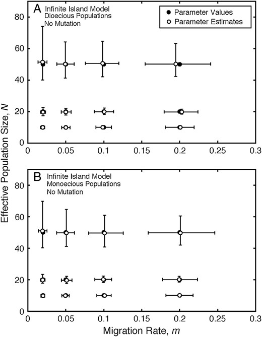
Infinite-island model: estimates of migration rate and effective population size. (A) Estimates of migration rate, m, and effective population size, N, under the infinite-island model with no mutation for different values of the migration rate and effective population size parameters for dioecious populations. (B) Estimates of migration rate, m, and effective population size, N, under the infinite-island model with no mutation for different values of the migration rate and effective population size parameters for monoecious populations. The medians (open circles) and interquartile ranges (error bars) of estimates of migration rate and effective population size from 400 replicate simulations are plotted for each pair of model values of migration rate and effective population size. Solid circles denote parameter values used to simulate the data.
Medians (5th, 95th percentiles) of the estimates of migration rate and effective population size using genotype data simulated under the infinite-island model at different values of migration rate, m, and effective population size, N, based on 400 replicate simulations for each pair of model migration rate and effective population size parameters for dioecious and monoecious model populations
Parameter estimates | |||||
|---|---|---|---|---|---|
| Parameter values | Dioecious populations | Monoecious populations | |||
| N | m | \({\hat{m}}\) | \({\hat{N}}\) | \({\hat{m}}\) | \({\hat{N}}\) |
| 10 | 0.02 | 0.019 (0.013, 0.027) | 9.91 (7.80, 13.22) | 0.019 (0.014, 0.027) | 9.73 (8.16, 12.46) |
| 0.20 | 0.200 (0.158, 0.248) | 9.96 (8.76, 11.88) | 0.199 (0.162, 0.244) | 10.05 (8.90, 11.29) | |
| 20 | 0.02 | 0.019 (0.012, 0.028) | 19.62 (15.04, 30.07) | 0.019 (0.012, 0.027) | 19.78 (15.33, 29.79) |
| 0.20 | 0.202 (0.152, 0.262) | 19.77 (16.47, 25.14) | 0.199 (0.147, 0.258) | 20.04 (16.36, 25.14) | |
| 50 | 0.02 | 0.019 (0.005, 0.032) | 51.39 (30.95, 172.5) | 0.019 (0.005, 0.033) | 50.90 (30.23, 165.7) |
| 0.20 | 0.194 (0.090, 0.322) | 50.18 (33.46, 101.9) | 0.200 (0.095, 0.322) | 49.66 (34.20, 95.17) | |
THE FINITE-ISLAND MODEL WITH k-ALLELE MUTATION
I now describe key results for the finite-island model with mutation following the k-allele mutation model; theoretical details are in the appendix. Under the finite-island model, s demes, each having effective population size N, exchange migrants at rate m, and genes can mutate into other alleles after gamete production according to the k-allele mutation model. The results that follow again apply to monoecious populations with no selfing and dioecious populations when males and females exhibit identical demography (including identical rates of mutation).
To verify the recursions in Equation 3, and thus that the estimators
The simulations of the finite-island model show, given sufficient data collected using a premigration census, that estimates of migration rate and effective population size using Equation 4 are close to their true values for both dioecious (Figure 2, A–C; Table 2) and monoecious populations (Figure 2D; Table 2). The precision of the estimates of N decreases with increasing values of N, and the precision of the estimates of m decreases with increasing values of m and N. The precision of the estimates of m and N decreases with lower mutation rates. Estimates of mutation rate, given sufficient data, are similarly close to their true values (Table 2). The precision of the estimates of u decreases with decreasing values of u and increasing values of N. Additional simulation results are in supplemental Table S2 at http://www.genetics.org/supplemental/.
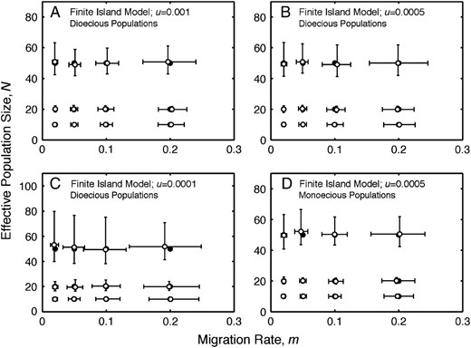
Finite-island model: estimates of migration rate and effective population size. (A) Estimates of migration rate, m, and effective population size, N, under the finite-island model for dioecious populations with u = 0.001. (B) Estimates of migration rate, m, and effective population size, N, under the finite-island model for dioecious populations with u = 0.0005. (C) Estimates of migration rate, m, and effective population size, N, under the finite-island model for dioecious populations with u = 0.0001. (D) Estimates of migration rate, m, and effective population size, N, under the finite-island model for monoecious populations with u = 0.0005. The medians (open circles) and interquartile ranges (error bars) of estimates of migration rate and effective population size from 400 replicate simulations are plotted for each pair of model values of migration rate and effective population size. Solid circles denote parameter values used to simulate the data.
Medians (5th, 95th percentiles) of the estimates of mutation rate, migration rate, and effective population size using genotype data simulated under the finite-island model with the k-allele mutation model at different values of mutation rate, u, migration rate, m, and effective population size, N, based on 400 replicate simulations for each pair of model migration rate and effective population size parameters for dioecious (u = 0.001, u = 0.0005, and u = 0.0001) and monoecious (u = 0.0005) model populations
Parameter values | Parameter estimates | |||
|---|---|---|---|---|
| N | m | \({\hat{u}}\) × 103 | \({\hat{m}}\) | \({\hat{N}}\) |
| Dioecious populations: k-allele mutation model, u = 0.001 | ||||
| 10 | 0.02 | 0.993 (0.693, 1.343) | 0.019 (0.013, 0.027) | 9.97 (8.36, 12.53) |
| 0.20 | 1.003 (0.716, 1.425) | 0.201 (0.155, 0.260) | 10.02 (8.60, 11.80) | |
| 20 | 0.02 | 1.005 (0.675, 1.348) | 0.020 (0.014, 0.026) | 20.09 (15.83, 26.87) |
| 0.20 | 1.005 (0.732, 1.371) | 0.202 (0.152, 0.257) | 19.92 (16.72, 24.95) | |
| 50 | 0.02 | 0.989 (0.523, 1.507) | 0.019 (0.011, 0.029) | 50.83 (35.17, 88.58) |
| 0.20 | 0.971 (0.569, 1.524) | 0.196 (0.112, 0.305) | 50.82 (35.10, 83.54) | |
| Parameter values | Parameter estimates | |||
| N | m | \({\hat{u}}\) × 104 | \({\hat{m}}\) | \({\hat{N}}\) |
| Dioecious populations: k-allele mutation model, u = 0.0005 | ||||
| 10 | 0.02 | 4.937 (3.299, 7.462) | 0.019 (0.014, 0.028) | 10.09 (8.12, 12.76) |
| 0.20 | 5.100 (3.287, 7.125) | 0.200 (0.144, 0.270) | 9.89 (8.50, 12.52) | |
| 20 | 0.02 | 5.038 (3.355, 7.123) | 0.020 (0.014, 0.026) | 19.97 (15.30, 27.83) |
| 0.20 | 4.914 (3.413, 7.067) | 0.198 (0.145, 0.265) | 19.86 (16.50, 25.72) | |
| 50 | 0.02 | 5.018 (2.529, 8.093) | 0.020 (0.010, 0.030) | 49.36 (33.45, 98.02) |
| 0.20 | 5.034 (2.521, 7.748) | 0.199 (0.098, 0.314) | 49.98 (34.53, 92.92) | |
| Dioecious populations: k-allele mutation model, u = 0.0001 | ||||
| 10 | 0.02 | 0.970 (0.423, 1.677) | 0.019 (0.010, 0.028) | 9.94 (7.59, 16.63) |
| 0.20 | 0.962 (0.354, 1.734) | 0.200 (0.105, 0.327) | 9.97 (7.47, 15.78) | |
| 20 | 0.02 | 0.977 (0.444, 1.610) | 0.019 (0.010, 0.030) | 19.68 (13.78, 35.61) |
| 0.20 | 1.025 (0.446, 1.824) | 0.198 (0.106, 0.339) | 19.92 (13.19, 35.27) | |
| 50 | 0.02 | 0.919 (0.096, 1.809) | 0.018 (0.002, 0.034) | 53.17 (29.94, 447.1) |
| 0.20 | 0.933 (0.250, 1.736) | 0.191 (0.056, 0.374) | 51.81 (31.04, 172.7) | |
| Monoecious populations: k-allele mutation model, u = 0.0005 | ||||
| 10 | 0.02 | 4.965 (3.299, 6.878) | 0.019 (0.014, 0.026) | 10.07 (8.69, 12.34) |
| 0.20 | 5.046 (3.356, 7.129) | 0.198 (0.151, 0.260) | 10.08 (8.77, 11.84) | |
| 20 | 0.02 | 4.985 (3.266, 7.065) | 0.020 (0.013, 0.027) | 19.83 (15.65, 27.23) |
| 0.20 | 4.836 (3.499, 7.004) | 0.196 (0.143, 0.266) | 20.17 (16.13, 26.19) | |
| 50 | 0.02 | 5.108 (2.216, 7.818) | 0.020 (0.009, 0.030) | 49.68 (33.53, 110.1) |
| 0.20 | 4.863 (2.877, 7.566) | 0.201 (0.113, 0.309) | 50.55 (35.33, 84.27) | |
Examples of the sampling distributions of the parameter estimates are shown in Figure 3 for dioecious populations with u = 0.0005, m = 0.05, and N = 20 for samples of 100 genotypes from 20 demes genotyped at 30 eight-allele loci. The distributions of
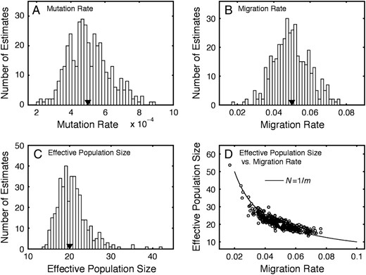
Sampling distributions of parameter estimates. (A) Sampling distribution of estimates of mutation rate, u. (B) Sampling distribution of estimates of migration rate, m. (C) Sampling distribution of estimates of effective population size, N. (D) Estimates of effective population size, N, graphed against estimates of migration rate, m. Estimates are from data simulated under the finite-island model for dioecious populations with k-allele mutation using parameters u = 0.0005, m = 0.05, and N = 20. Triangles denote values of the parameters.
In empirical situations, k, the number of possible alleles at a locus, might be expected to vary across loci. In this case, estimates of u, m, and N may be constructed from the moment equations defined by summing the left- and right-hand sides of Equation 4 over loci and setting the left-hand sum equal to the right-hand sum. Simulations of dioecious populations in the finite-island model (100 individuals genotyped from each of 20 demes) with k-allele mutation (u = 0.0005) for 30 loci having a random mixture of 4, 8, or 12 possible alleles show, given sufficient data collected using a premigration census, that estimates of mutation rate, migration rate, and effective population size are close to their true values and have similar properties to those calculated when all loci have the same number of possible allelic states (simulation results are in supplemental Table S3 at http://www.genetics.org/supplemental/).
ROBUSTNESS OF THE ESTIMATION PROCEDURES
The extent to which a statistical procedure yields useful parameter estimates typically depends on the appropriateness of the assumptions to a given data set. Accordingly, I assessed the properties of the parameter estimates when some of the assumptions of the models are violated.
I used the k-allele mutation model to describe the mutation process in the estimation procedure described above. The infinite-allele model (Kimura and Crow 1964) can be employed using Equation 4 by setting k to a large (and effectively infinite) value. An alternative mutation model that may be appropriate for some markers such as microsatellite sequences is the stepwise mutation model (Ohta and Kimura 1973). The stepwise mutation model assigns a length-based ordering to alleles and posits that mutation occurs between allelic states that are adjacent in the ordering. Accordingly, I applied the estimation procedure to data generated using the simulation approach described above for the finite-island model except that I implemented mutation according to two simple kinds of stepwise mutation models: a stepwise mutation model with no bounds on allele length (unbounded stepwise mutation model; Ohta and Kimura 1973) and a stepwise mutation model with lower and upper bounds on allele length (bounded stepwise mutation model; constrained to eight allelic states). I simulated genotype data under the finite-island model with dioecious populations over a range of migration rates (0.02, 0.05, 0.10, and 0.20) and effective population sizes (10, 20, and 50) at a mutation rate of u = 0.0005. Hence, each generation every gene mutates to an adjacent allele with probability u, mutating to either neighboring allele with equal probability. In the bounded stepwise mutation model, genes at the lower bound mutate toward the upper bound and genes at the upper bound mutate toward the lower bound. The simulations were carried out using 30 independent eight-allele loci (with equally frequent alleles) at which 100 offspring were genotyped from each of 20 demes after 6000 generations. Simulated data were combined over loci to calculate
The accuracy (when comparing the medians of replicate estimates to their parametric values) of estimates of migration rate and effective population size for data generated under the stepwise mutation models is similar to that observed under the k-allele mutation model (Figure 4; Table 3), despite the fact that the k-allele mutation model is the assumed mutation process in Equation 4. In particular, the medians of the estimates of m and N are close to their respective parametric values. The estimates of m and N for data generated under the stepwise mutation models (Figure 4; Table 3) exhibit levels of precision similar to, but slightly lower than, the estimates of those parameters for data generated under the equivalent k-allele mutation model (Figure 2B; Table 2). Hence, the estimates of m and N based on Equation 4 are somewhat robust to violations in the assumptions of the mutation model. In contrast, the estimates of mutation rate, when summarized using their medians, are negatively biased (Table 3), suggesting that the mutation rate estimates are sensitive to violations in the assumptions of the mutation model in the estimation procedure. Additional simulation results are in supplemental Table S4 at http://www.genetics.org/supplemental/.
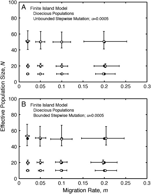
Finite-island model: stepwise mutation models. (A) Estimates of migration rate, m, and effective population size, N, under the finite-island model with unbounded stepwise mutation for different values of the migration rate and effective population size parameters for dioecious populations. (B) Estimates of migration rate, m, and effective population size, N, under the finite-island model with bounded stepwise mutation for different values of the migration rate and effective population size parameters for dioecious populations. The medians (open circles) and interquartile ranges (error bars) of estimates of migration rate and effective population size from 400 replicate simulations are plotted for each pair of model values of migration rate and effective population size. Solid circles denote parameter values used to simulate the data.
Medians (5th, 95th percentiles) of the estimates of mutation rate, migration rate, and effective population size using genotype data simulated under the finite-island model with stepwise mutation models (employing either unbounded or bounded ranges in allele lengths; u = 0.0005) at different values of migration rate, m, and effective population size, N, based on 400 replicate simulations for each pair of model migration rate and effective population size parameters for dioecious model populations
Parameter values | Parameter estimates | |||
|---|---|---|---|---|
| N | m | \({\hat{u}}\) × 104 | \({\hat{m}}\) | \({\hat{N}}\) |
| Dioecious populations: unbounded stepwise mutation model, u = 0.0005 | ||||
| 10 | 0.02 | 3.712 (2.619, 5.420) | 0.020 (0.014, 0.028) | 10.00 (8.02, 13.15) |
| 0.20 | 4.189 (2.862, 6.108) | 0.197 (0.152, 0.268) | 10.06 (8.36, 12.26) | |
| 20 | 0.02 | 3.600 (2.385, 4.965) | 0.020 (0.013, 0.028) | 19.79 (15.21, 28.11) |
| 0.20 | 3.798 (2.431, 5.489) | 0.202 (0.136, 0.278) | 19.91 (15.87, 28.06) | |
| 50 | 0.02 | 2.898 (1.316, 4.757) | 0.020 (0.009, 0.031) | 51.23 (32.43, 107.5) |
| 0.20 | 3.066 (1.492, 4.841) | 0.198 (0.092, 0.333) | 50.63 (33.15, 108.2) | |
| Dioecious populations: bounded stepwise mutation model, u = 0.0005 | ||||
| 10 | 0.02 | 3.409 (2.254, 5.292) | 0.020 (0.013, 0.027) | 9.95 (7.88, 13.48) |
| 0.20 | 3.731 (2.335, 5.678) | 0.202 (0.145, 0.264) | 9.97 (8.31, 12.78) | |
| 20 | 0.02 | 3.286 (1.967, 4.810) | 0.020 (0.013, 0.029) | 19.73 (14.78, 30.14) |
| 0.20 | 3.306 (1.968, 5.042) | 0.197 (0.129, 0.286) | 20.22 (15.31, 29.01) | |
| 50 | 0.02 | 2.652 (1.183, 4.584) | 0.019 (0.008, 0.032) | 53.26 (32.71, 119.4) |
| 0.20 | 2.861 (1.224, 4.730) | 0.203 (0.092, 0.327) | 50.36 (33.12, 103.7) | |
The assumption of temporal equilibrium in the probability of identity recursion equations is used to estimate mutation rate, migration rate, and effective population size. To assess this assumption, I applied the estimation procedure to genotype data simulated under nonequilibrium conditions using the infinite-island model with no mutation and the finite-island model with mutation for dioecious populations with parameter values m = 0.05 and N = 20. For the finite-island model, I simulated data under the k-allele mutation model, the unbounded stepwise mutation model, and the bounded stepwise mutation model using a mutation rate of u = 0.0001 (the value of the mutation rate requiring the most generations to reach temporal equilibrium). At these parameter values, the infinite-island model is very close to temporal equilibrium after 50 generations, whereas the finite-island model with k-allele mutation requires ∼10,000 generations to reach equilibrium to four decimal places. Diploid genotypes were initialized using random pairs of alleles, the life cycle was iterated for 10, 20, 50, 100, or 200 generations, and genotypes were then sampled prior to migration (100 offspring genotyped at 30 eight-allele loci in each of 20 demes).
The accuracy of the estimates of mutation rate, migration rate, and effective population size, measured using the median of replicate estimates relative to their parametric values, increases as the number of generations increases from 10 to 200 for both the infinite- and the finite-island models (Figure 5). The estimates of u under the finite-island models are strongly positively biased at 10–200 generations (Figure 5A). In contrast, the estimates of m under the infinite-island model and the finite-island model with unbounded stepwise mutation are positively biased at 10 generations, but are nearly unbiased after ≥20 generations (Figure 5B). The estimates of m under the finite-island models with k-allele and bounded stepwise mutation models are negatively biased, but the bias is relatively small, especially after ≥100 generations (Figure 5B). The estimates of N exhibit the least bias among the estimated parameters, indicating essentially no bias in the infinite-island model and the finite island model with unbounded stepwise mutation at ≥10 generations and a small negative bias in the finite-island models with k-allele and bounded stepwise mutation models after 10 and 20 generations and very little bias for ≥50 generations (Figure 5C). The precision (measured via 5th and 95th percentiles in Figure 5) of the estimates of m and N is high relative to estimates of those parameters under equilibrium conditions (see supplemental Table S2 at http://www.genetics.org/supplemental/: u = 0.0001, m = 0.05, N = 20). Hence, the estimation procedures do not require equilibrium conditions to provide reasonable estimates of migration rate and effective population size, and the nonequilibrium conditions explored here actually increase the precision of these estimates. In contrast, the nonequilibrium conditions examined here result in inaccurate estimates of the mutation rate. Simulations suggest that at least 4000 generations under the finite-island model with k-allele mutation are required to obtain accurate estimates of the mutation rate when u = 0.0001, m = 0.05, and N = 20.
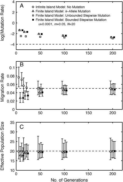
Estimation under nonequilibrium conditions. (A) Estimates of mutation rate, u, (on the log scale) as a function of number of generations using data generated under finite-island models with different mutation models for dioecious populations. (B) Estimates of migration rate, m, as a function of number of generations using data generated under the infinite-island model with no mutation and finite-island models with different mutation models for dioecious populations. (C) Estimates of effective population size, N, as a function of number of generations using data generated under the infinite-island model with no mutation and finite-island models with different mutation models for dioecious populations. The medians (symbols) and 5th and 95th percentiles (error bars) of estimates from 400 replicate simulations are plotted for each model at generations 10, 20, 50, 100, and 200. Dashed lines denote the parameter values u = 0.0001, m = 0.05, and N = 20. Symbols have been offset along the x-axis to improve clarity.
The estimation of parameters using Equation 4 assumes that k, the number of possible allelic states at a locus, is known. In practice, k might be estimated using the total number of alleles observed in all of the data for each locus, and there would be uncertainty in its value. Accordingly, using data generated under the finite-island models (100 offspring genotyped at 30 eight-allele loci in each of 20 demes after 6000 generations; hence k = 8) with k-allele mutation, unbounded stepwise mutation, and bounded stepwise mutation (u = 0.0005, m = 0.05, N = 20), I calculated estimates of mutation rate, migration rate, and effective population size using values for k in Equation 4 equal to 2, 4, 8, 16, and 100.
The medians of the estimates of migration rate and effective population size are close to their parametric values over the range of assumed values of k (2, 4, 8, 16, and 100), but the medians of the estimates of mutation rate deviate from the parametric values for most of the assumed values of k, with most cases exhibiting negative bias. The precision (measured via 5th and 95th percentiles) of the estimates of m and N is similar over the range of assumed values of k with the exception that estimates of m are slightly less precise for k = 2 under the k-allele mutation model. Estimates of u for k = 2 are quite variable and some are very near zero; otherwise the precision of the estimates of u is similar across the different assumed values of k. Hence, estimates of m and N are robust to uncertainty in the value of k, and, in contrast, estimates of u are more sensitive to deviations from the parametric value of k.
DISCUSSION
Population geneticists have actively studied the idea that demographic parameters such as migration rate and effective population size might be estimable from genetic data (e.g., Slatkin 1985; Waples 1989; Pudovkin et al. 1996; Beerli and Felsenstein 2001; Vitalis and Couvet 2001; Wang and Whitlock 2003; Robledo-Arnuncio et al. 2006). Using the classic island model (Wright 1951), I report that migration rate and effective population size can be jointly estimated from probabilities of identity using neutral markers in dioecious or monoecious populations when offspring genotypes are collected prior to migration from a single generation at a single point in time. The life cycle and sampling model are appropriate for highly fecund organisms with localized mating, including species of invertebrates, amphibians, fishes, and plants; hence the method has the potential for broad taxonomic utility.
The estimation procedure works because assuming a dioecious population—or monoecious populations with no selfing—in which offspring genotypes are sampled prior to migration has the consequence that Q1(t) ≠ Q2(t) and hence provides additional information that is not available for other mating systems and sampling schemes that result in Q1(t) = Q2(t) (e.g., random selfing resulting in random pairing of gametes from all adults during mating, including pairing of gametes from the same adult; Maruyama 1970; Nei and Feldman 1972; Nagylaki 1983; Crow and Aoki 1984; Epperson 1999) or Q1(t) very nearly equal to Q2(t) (e.g., the finite-island model under a postmigration census). Previous studies in population ecology (e.g., Caswell 2001) and genetics (e.g., Nagylaki 1983; Waples 1989; Vitalis 2002) have recognized that the mating system and/or timing of sampling can affect the interpretation of demographic quantities, but the application of these ideas to the present scenario of joint estimation of migration rate and effective population size using a sample from a single generation collected at a single point in time seems not to have been analyzed in prior investigations. Several studies have examined recursions for probabilities of identity in state that are similar to those used here, but these studies do not identify the estimation procedures developed here. In the appendix, I outline how various recursions for probabilities of identity that have been studied (Maruyama 1970; Maynard Smith 1970; Nei and Feldman 1972; Nagylaki 1983; Crow and Aoki 1984; Epperson 1999; Vitalis and Couvet 2001; Vitalis 2002; Balloux et al. 2003) can be derived under the pre- and postmigration census schemes, thus helping to explain the different forms of these equations that occur in the literature. Indeed, Vitalis and Couvet (2001) estimate m and N using probabilities of identity, and their Equation 5 with no selfing is equivalent to the infinite-island model with k-allele mutation under a premigration census as defined here; but Vitalis and Couvet (2001) assume an infinite-island model with mutation among an infinite number of alleles, and they use the approximation
Like other genetic methods for estimating demographic parameters (e.g., Waples 1989; Pudovkin et al. 1996; Williamson and Slatkin 1999; Beerli and Felsenstein 2001; Vitalis and Couvet 2001; Wang and Whitlock 2003), the procedure described here will typically require considerable data to recover accurate and precise estimates. The accuracy and precision achieved will, in general, depend on several factors, including the values of the parameters u, m, and N, as well as the number of demes, number of individuals genotyped, number of loci used, and the appropriateness of the model to the empirical system under investigation. Previous studies (Waples 1989; Pudovkin et al. 1996; Williamson and Slatkin 1999; Vitalis and Couvet 2001; Wang and Whitlock 2003) have shown that effective population size is more difficult to estimate as N increases, and my simulation results are consistent with the findings in these earlier studies. Indeed, my results suggest that Q1(t) and Q2(t) become increasingly similar as N increases, with the consequence that estimates of N approach infinity as
The simulation results suggest that the estimates of migration rate and effective population size are somewhat robust to violations of the model assumptions. Reasonable estimates of m and N can be obtained for loci exhibiting stepwise mutation (Ohta and Kimura 1973), under nonequilibrium conditions, or if the number of possible allelic states is not precisely known. In contrast, estimates of the mutation rate, u, are sensitive to violations in the assumptions and can be quite biased in these settings. The precision of the estimates of m and N is higher for data simulated with a high mutation rate and for data simulated under nonequilibrium conditions, suggesting that the procedure works better at higher levels of genetic diversity. The estimation procedure under the finite-island model requires that the number of demes, s, be known, but it does not require that all demes be sampled because all demes are identical in island models. In non-island models, the set of demes that is exchanging migrants generally must be known to estimate migration rates among the demes (Beerli and Felsenstein 2001; Wang and Whitlock 2003; Slatkin 2005).
Many studies investigate the estimation of demographic parameters from genetic data (Slatkin 1985; Waples 1989; Pudovkin et al. 1996; Wang and Whitlock 2003; Robledo-Arnuncio et al. 2006); however, few methods exist for jointly estimating parameters like migration rate and effective population size from genetic data collected from a sample taken from a single generation at a single point in time (Beerli and Felsenstein 1999, 2001; Vitalis and Couvet 2001). For example, the product parameter mN can be estimated from single-generation data on FST under the infinite-island model (Slatkin 1985), and effective population size alone can be estimated from multiple samples on allele frequencies from two or more generations (Waples 1989) or from a single sample of offspring assuming unrelated parents using heterozygote excess (Pudovkin et al. 1996). Vitalis (2002) and Fontanillas et al. (2004) use two samples (both pre- and postmigration samples) to estimate migration rate alone using F-statistics under the infinite-island model with sex-specific dispersal. Extending the idea in Waples (1989), if allele frequency data are available from multiple samples from multiple generations from two or more demes, then migration rate and effective population size can be jointly estimated (Wang and Whitlock 2003). Using data from a single generation, the method of Beerli and Felsenstein (2001) estimates the deme-specific product parameters 4uN and m/u for s demes under a general migration scheme under the assumption that effective population size is sufficiently large so that the coalescent model of genetic drift is appropriate and that m and u are sufficiently small so that the quantities mN and uN remain finite as N goes to infinity. In a two-deme version of their coalescent procedure, Beerli and Felsenstein (1999) initially estimate 4uN and m/u using moment estimators based on the probability-of-identity equations of Nei and Feldman (1972), which can be derived for randomly mating monoecious populations under a postmigration census scheme. The method of Vitalis and Couvet (2001) uses one- and two-locus probabilities of identity to estimate m and N under the infinite-island model with infinite-allele mutation and random selfing, assuming that u = 0 and m is sufficiently small so that the approximation
The method I describe here requires only a sample from a single generation at a single point in time; it can jointly estimate mutation rate, migration rate, and effective population size; it is relatively simple computationally and, given the parametric model, need not make assumptions concerning the values of parameters that might be estimated; but, at present, it has not been developed to accommodate more general demographic situations. However, it may be possible to extend the method to include other demographic and genetic scenarios, such as a time series of samples (Wang and Whitlock 2003), stepping-stone dispersal, more general migration models (e.g., Beerli and Felsenstein 2001), deme-specific effective population sizes, and other mutation models (e.g., Lai and Sun 2003). More general forms of the model can lead to additional (but still linear) recursions for the probabilities of identity in state, but if the probability of identity within individuals remains different from the probability of identity among individuals within demes in these more general settings, then information may be available to jointly estimate migration rates and effective population sizes in more detailed models.
APPENDIX
I consider parametric expressions involving Q1(t), Q2(t), and Q3(t), the probabilities of identity in allelic state within one selectively neutral locus at time t, in an s-deme finite-island model with genetic drift, migration, and mutation. I adopt part of the derivation strategy of Nagylaki (1983) and outline the life cycle for the models that I consider. Starting with N diploid, monoecious adults in each of s demes, reproduction begins with each adult producing a large (i.e., infinite) number of haploid gametes. The allele in each gamete may then mutate into a different allele according to a general mutation model. The reproduction phase is completed by the random pairing of gametes from different adults within demes; no offspring are produced using two gametes from the same adult (i.e., no selfing occurs). Offspring then migrate among demes so that, following migration, a fraction m of the individuals in a deme are migrants and a fraction 1 − m of the individuals are residents. Population regulation completes the life cycle with N offspring chosen at random within each deme to compose the adults that will produce the next generation. The life cycle just described is the diploid dispersion life cycle considered by Nagylaki (1983). The equilibrium results that follow also apply to dioecious populations when males and females are equal in number (the populations within demes are regulated to N/2 females and N/2 males so that the total adult effective population size is N), migrate at the same rate, and experience the same mutation model.
Because demographic and genetic measures can depend on the timing of sampling within the life cycle (e.g., Waples 1989; Caswell 2001; Vitalis 2002), I consider two census schemes, a premigration census and a postmigration census. Assuming pre- and postmigration census schemes for dioecious populations with sex-specific dispersal following the infinite-allele mutation model in a finite number of demes, Vitalis (2002) gives recursions for probabilities of identity by descent (premigration, Equation A1.4; postmigration, Equation A1.1; Vitalis 2002) that can be readily modified to obtain the results that follow. Note that the second and third columns in the matrix A following Equation A1.1 in Vitalis (2002) should have terms like (1 − 2/N) consistent with Equation 4 in that article, rather than terms like (1 − 1/N).
Probabilities of gene identity have been analyzed extensively in the population genetics literature. I briefly summarize previous results in the context of the models that I have presented here. Equation 2-1 of Maruyama (1970) and Equation 1 of Nei and Feldman (1972) can be derived in the present context by assuming a finite-island model, mutation among an infinite number of alleles, and monoecious populations with random mating [including random selfing; hence, Q1(t) = Q2(t)] under a postmigration census. Equation 78 of Nagylaki (1983) with zero selfing can be derived by assuming a finite-island model, mutation among an infinite number of alleles, and monoecious populations with no selfing under a postmigration census. Equation 5 of Crow and Aoki (1984) can be derived by assuming a finite-island model, mutation among k alleles, and monoecious populations with random mating [including random selfing; hence, Q1(t) = Q2(t)] under a postmigration census. Equation 2 of Epperson (1999) can be derived by assuming a finite-island model with general between-deme migration rates, no mutation, and monoecious populations with random mating under a postmigration census. Recursions for Q1(t) and Q3(t) [a one-generation recursion for Q2(t) is not presented] in Maynard Smith (1970) can be derived by assuming a finite-island model, mutation among an infinite number of alleles, and monoecious populations with no selfing under a premigration census. Equation 5 of Vitalis and Couvet (2001) with zero selfing can be derived by assuming an infinite-island model, mutation among k alleles, and monoecious populations with no selfing under a premigration census. Equations A1.1 and A1.4 of Vitalis (2002), assuming pre- and postmigration census schemes, respectively, can be derived assuming dioecious populations with sex-specific dispersal following the infinite-allele mutation model in a finite number of demes. Finally, the juvenile life stage recursions of Balloux et al. (2003) with no selfing and no clonal reproduction can be derived by assuming a finite-island model, mutation among an infinite number of alleles, and monoecious populations with no selfing under a premigration census. Although many previous studies have analyzed probabilities of gene identity, I am not aware of any study that has identified the connection between the census scheme and the procedures for estimating mutation rate, migration rate, and effective population size as I have outlined them here.
Footnotes
Communicating editor: R. Nielsen
Acknowledgement
I thank Mark Holder, Steve Hudman, John Kelly, Rasmus Nielsen, Bruce Weir, and two anonymous reviewers for assistance, conversations, and/or comments concerning this research. I acknowledge funding from the University of Kansas and the National Science Foundation (DEB 06-09722).
References
Beerli, P., and J. Felsenstein,
Caswell, H.,
Crow, J. F., and K. Aoki,
Maynard Smith, J.,
Nagylaki, T.,
Rousset, F.,
Slatkin, M.,
